
Department of Mathematics Education

This exploration with graphs of mathematical relations grew out of some
class discussions with prospective teachers as we examined the use of the
computer for graphing mathematical relations. The use of the computer allows
us to explore and conjecture and develop ideas with respect to the mathematical
relations and their graphs.
The particular relation was
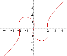
Cursory discussion led to agreement that the curve would cross the y-axis
at three points -- -1, 0, and 1 -- and likewise the curve would cross the
x-axis at three points -- -2, 0, and 2. Also, for large x, y is large, etc.
The computer provides a tool to draw the graph, look closely at particular
regions of the graph, and so forth. It was clear that the interesting part
of the graph would be near the origin. Using Algebra Xpresser (Hoffer, 1989)
the graph was obtained as follows.
A point of discussion was to explore changes in the graph that resulted
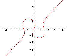
from changes in the relation. For example, the following resulted when the
4 on the right hand side was change to 2. The curve as a somewhat similar
shape but is more compressed, crossing the x-axis at points closer to the
origin.
Why not go further and see what happens when the constant on the right
hand side is 1, producing a relation symmetric with respect to x and y?
Surely the symmetry will add some demand to the graph. The result is the
following.
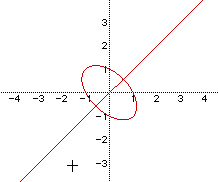
The graph now looks like the composite of two graphs -- a line and an
ellipse. It is a single relation, but some algebra -- either
by hand or by symbol manipulator -- can lead to a factored form of the equation,
and one factor corresponds to the line and the other corresponds to the ellipse.
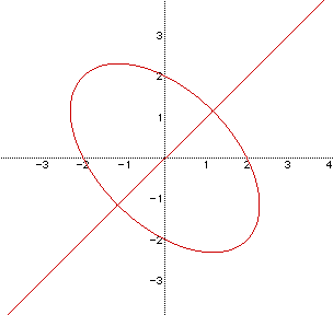
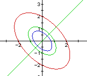
is an ellipse with major axis along the line y = -x and contains the
points (0,2),
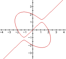
(0,-2), (2,0), and (-2,0). A graph is in Figure 1.

Next, consider any line with a graph passing through this ellipse. A
simple case would be y = x. But, rather than graphing the ellipse and then
the line as an overlay, consider the following relation
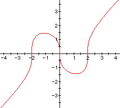
The graph of this relation will be the ellipse and the line through it.
Figure 2 is a graph of the new relation.
Using some algebra, this latter relation is transformed into
A family of curves can be generated by considering
where a and b are real numbers. In fact, if a = b and both are positive,
then all that changes from Figure 2 to a new graph is scaling. For example,
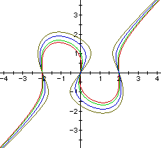
the three graphs

are shown in Figure 3.
Much more interesting, however, are the curves where a and b are not
equal. For example, in Figure 4, a = 3 and b = 4.

In Figure 5, a = -4 and b = 4.

In Figure 6, a = 0 and b = 4.
In Figure 7, graphs for a = .5, 1, 2, and 3 are given for b = 4 in each
case. In Figure 8, the values of a and b are reversed.
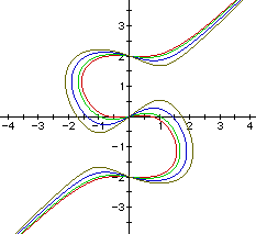

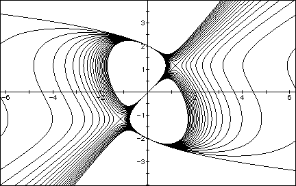
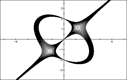
Figures 11 and 12 each show a set of curves that can be produced by varying
different coefficients. Each is a set of 21 graphs where a coefficient has
been stepped over 2 units in steps of 0.1. Figure 11 varies the coefficient
of the ![]() term from 0 to 2; Figure 12 varies the coefficient of x from 3 to 5.
term from 0 to 2; Figure 12 varies the coefficient of x from 3 to 5.
If we rewrite the equation as
the three-dimensional graph would be a surface -- much like an undulating
blanket looping through the origin (0,0,0)
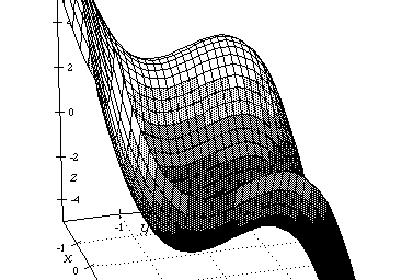
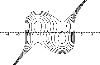
Now, to examine cross-sections where z = -3, -2, -1, 0, 1, 2, 3 gives
the
following graphs (contour lines?):
There is more to the investigation of these curves stimulated by the
look at this equation, but let us turn our attention to applying the technique
of multiplying relations to build composite curves that can in turn be modified
to build a family of curves. Consider a very simple case, beginning with
the equations for two lines:
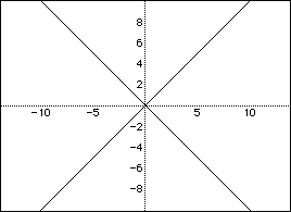
The product of the two relations is
and the graph is
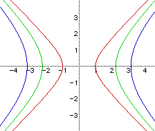
If the product is set equal to some constant other than 0, the graph
is a hyperbola from the family of hyperbolas having these two lines as asymptotes.
The following graph shows the graphs for three hyperbolas in this family.
Similarly, if any other lines were selected, the technique could generate
a family of hyperbolas.
The technique can be used to build families of curves for which new conjectures
and problems can be formed. For example, if the component curves are two
overlapping ellipses, then the entire family of curves may be bounded. It
is illustrative, but not necessary, to examine inequalities rather than
equations. Let the product be

and multiply the factors in the left hand side to get
If the constant term is replaced by 15 or by 17, the following graphs
are found. It is illustrative, but not necessary, to examine inequalities
rather than equations.
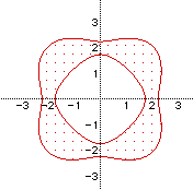
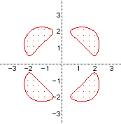
As the constant term is replaced by numbers lower than 15 the region
in the center gets smaller and the shape approaches a square with the corners
rounded. When will the center region reduce to a point? Why?
As the constant term is replaced by numbers larger than 17 the four small
regions get smaller. When will they reduce to four points? What are the
points? Why?
Finally, one more problem . . .What is the equation for the following graph?
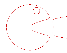
Does this help?
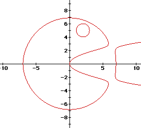
I used
for the large circle and
for the horizontal parabola. Their product and expansion are
Now, replace the second coefficient of 49 with 47 to separate the intersections
points in the graph and multiply this expression by an espression for the
small circle representing the eye.
Experiment with other replacements of this coefficient, or others in
the expression, to see variations in the result.