
A parametric curve in the plane is a pair of functionsx = f(t)
y = g(t)
where the two continuous functions define ordered pairs (x,y). The two equations are usually called the parametric equations of a curve. The extent of the curve will depend on the range of t and your work with parametric equations should pay close attention the range of t . In many applications, we think of x and y "varying with time t " or the angle of rotation that some line makes from an initial location.
Various graphing technology, such as the TI-81, TI-82, TI-83, TI-84,TI-85, TI-86, TI-89, TI- 92, and Graphing Calculator 3.5 or 4.0 can be readily used with parametric equations. Try Graphing Calculator 3.5 or GC 4.0 for what is probably the friendliest software. Geogebra and Desmos can also deal with parametric curves. Graphing Calculator 4.0 Lite DOES NOT handle parametric equations.Note: Graphing technologies compute values of (x,y) for increments of t and then construct a line segment connecting them. When the increment of t is small these are very short segments and the curve is simulated. The TI instruments include a 'step' setting for the increments of 't' and it is possible for consecutive (x,y) to be rather far apart. This can produce interesting drawings but misrepresent the parametric curve given by the set of points. In other words, the 'step' setting is a way of drawing segments between regularly spaced but not adjacent points on the parametric curve.
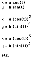
1. Graph

How would you change the equations to explore other graphs?
2. For various a and b, investigate
3. For various a and b, investigate

4. Graph

Interpret. What would you change to explore and understand the graphs?
5. Graph several sets of curves for

for selected values of a, b, and k in an appropriate range for t. (Set a and b and then overlay graphs for several values of k. Repeat for new values of a and b.)
6. Graph

for some appropriate range for t.
Interpret. Is there anything to vary to help understand the graph?
7. Write parametric equations of a line segment through (7, 5) with slope of 3. Graph the line segment using your equations. As a line segment, it will have end points. Explore how you would choose endpoints of such that the two distances from (7, 5) are 2 units and 3 units.
8. Investigate

for different values of a and b. What is the curve when a < b? a = b? a > b?
Describe fully. What is changed if the equations are

where h is any real number?
Investigate with graphs for small h (e.g. -3 < h < 3).
NOTE: These latter parametric equations describe the locus of the vertex (x,y) of a triangle with altitude h whose other two vertices are moved, one along the x-axis and the other along the y-axis.
9. Derive the parametric equations for the locus of a point (x, y) on a line segment that is moved so that one end is on the x-axis and the other end is on the y-axis.
10. Investigate each of the following for

Describe each when a = b, a < b, and a > b.

11. Consider

The equation is easy to graph with Graphing Calculator 3.5 or 4.0 but would be difficult to graph with most Function Grapher applications. Putting it in parametric form makes it possible to graph with many other applications (including the TI-81 or TI-82).
Let y = tx cross the curve at (0,0) and at (x,y). Then, substituting,

and so we have the parametric equations

Graph the curve using the parametric equations for a suitable range of t.
Graph

using Graphing Calculator 3.5 or 4.0 for comparison.
12. Investigation. Consider the parametric equations

Graph these for

Describe fully. You may have to increase the range of t for the larger fractions. This class of parametric curves are called the Lissajous curves. Compare with
x = sin((a)t)
y = sin((b)t)
13. A cycloid is the locus of a point on a circle that rolls along a line. Write parametric equations for the cycloid and graph it. Consider also a GSP construction of the cycloid. Click HERE to see a GSP animation showing the cycloid.
Click HERE for a derivation of parametric equations for the cycloid.