

We will be exploring the graph of the above equation. Most students will know what the graph of a parabola looks like.
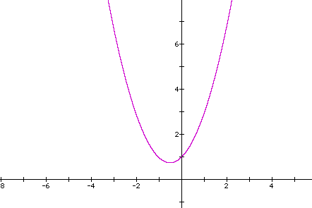
We will be using Graphing Calculator 3.0 to explore different forms of this equation. We will vary a and b to see the different types of graphs. Many students have a difficult time visualizing different graphs at the same time. For example, if I were to ask my students, "what happens when we change the a in the following equation:
We can use Graphing Calculator 3.0 to graph different values on the same axis so that the student can see exactly what happens. In the following graph I have varied a from -3 to 3. For each value and its negative I have color coordinated them together. (i.e. when a = -3 and 3 the graph is blue)
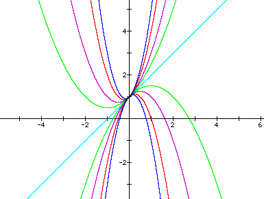
This will allow students to see what each variation will look like. Being able to visualize ideas will create confidence in your students. We can also ask another question, "What is the locus of vertices of the different parabolas?" Well, here it is not very difficult to see: a single point. For each parabola the vertex is the same.
Next let's look at varing b. We can ask the same questions about this variable.
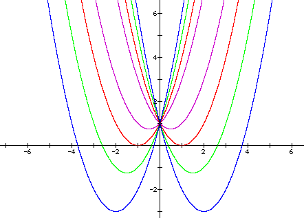
What is the locus of points for the vertices of each of the parabolas here? Some students may be able to see right away that it is a parabola pointing down with its vertex at (0,1). Other students may not be able to see so quickly. Graphing Calculator 3.0 has an animation function that is really cool. This will allow the student to see, as the graph changes, where the vertex lies.
Click here to see the animation of the variable b.
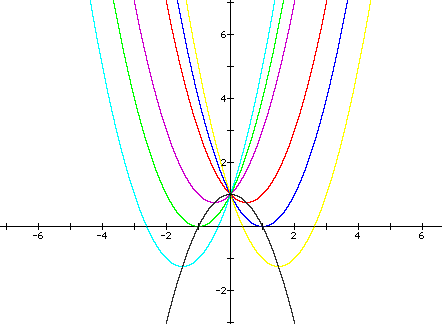
As shown in the above graph we can clearly see that the locus is a parabola. Interacting with the graphs will help students become much more confident in their mathematics. Another topic we will discuss will be roots. When I learn roots for the first time it took a little while for the information to sink into my brain. We are going to talk about looking at these graphs in the xb plane. It is a bit strange at first but it helps to show roots of these equations.
Consider the following equation
When we graph this in the xb plane we will get the following graph.
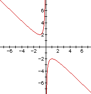
If we take any particular value of b, say b=3, and overlay this equation on the graph we add a line parallel to the x-axis. If it intersects the curve in the xb plane the intersection points correspond to the roots of the original equation for that value of b. We have the following graph.
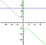
For each value of b we select, we get a horizontal line. It is clear on a single graph that we get two negative real roots of the original equation when b>2, one negative real root when b=2, no real roots for-2<b<2, one positive real root when b=-2, and two positive real roots when b<-2.
This is another way of looking at explaining roots of a quadratic equation.