
The assignment for this write-up was to use historical data for the price of stamps to formulate a function to fit a line to the historical data and to be used as a prediction function for future price increases.
The data was collected in an Excel file and is as follows:
| YEAR | PRICE(in cents) |
| 1919 | 2 |
| 1932 | 3 |
| 1958 | 4 |
| 1963 | 5 |
| 1968 | 6 |
| 1971 | 8 |
| 1974 | 10 |
| 1975 | 13 |
| 1978 | 15 |
| 1981 | 20 |
| 1985 | 22 |
| 1988 | 25 |
| 1991 | 29 |
| 1994 | 32 |
| 1997 | 33 |
| 1999 | 34 |
| 2002 | 37 |
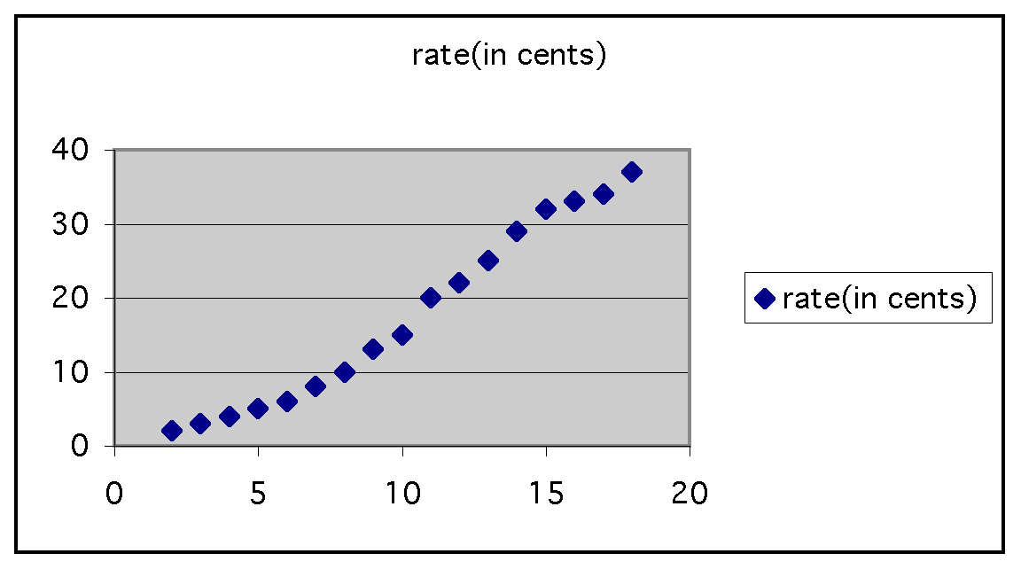
To understand the type of relationship between the dependent (the price of stamps) and independent (the year) variables, let's plot a graph of this data and see the shape it takes. For instance, if this graph can take the shape of a straight line, we would know that the relationship between the two variables is linear.

It's important to note here that if we plot only the price changes as listed in the table given above, the graph (as we see above) does not reflect the differences in the number of years lapsed between price increases.
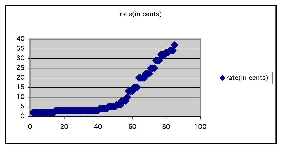
We can adjust for this by creating a table that lists the price data for intermediate years.
Here is a picture of the graph with adjustments made to reflect the time lapses between rate increases:

The graph above is a more accurate illustration of the relationship between time and the price of stamps. We can also see from the graph that the relationship is more likely to be exponential than it is to be linear. For this reason, instead of finding an equation to fit the linear form of :
price = x*(number of years) + c
We will focus on the form :
price = x^(a*number of years)+c
Because our initial price is 2 cents, let's start by looking at the estimates we would derive from an exponential equation that used the form:
price = 2*A^(current year - 1919), where A would be the average ratio of change-to-change prices
(For now let's start with A close to 1. We'll assign the value A=1.1 and see what this creates:
| YEAR | RATE(in cents) | Estimated Rate | Absolute Difference |
| 1919 | 2 | 2 | 0 |
| 1932 | 3 | 6.90454242878621 | 3.90454242878621 |
| 1958 | 4 | 82.289555578502 | 78.289555578502 |
| 1963 | 5 | 132.528152154733 | 127.528152154733 |
| 1968 | 6 | 213.437914326719 | 207.437914326719 |
| 1971 | 8 | 284.085863968864 | 276.085863968864 |
| 1974 | 10 | 378.118284942558 | 368.118284942558 |
| 1975 | 13 | 415.930113436813 | 402.930113436813 |
| 1978 | 15 | 553.602980984399 | 538.602980984399 |
| 1981 | 20 | 736.845567690235 | 716.845567690235 |
| 1985 | 22 | 1078.81559565527 | 1056.81559565527 |
| 1988 | 25 | 1435.90355781717 | 1410.90355781717 |
| 1991 | 29 | 1911.18763545465 | 1882.18763545465 |
| 1994 | 32 | 2543.79074279014 | 2511.79074279014 |
| 1997 | 33 | 3385.78547865368 | 3352.78547865368 |
| 1999 | 34 | 4096.80042917095 | 4062.80042917095 |
| 2002 | 37 | 5452.84137122654 | 5415.84137122654 |
Clearly we have assigned a wrong value somewhere...!
Let's go back and look at the ratios of prices, where the new price year n+x is compared to the price of year n. For example, what is the ratio of the price of stamps in 2002 to the price of stamps1999?
| YEAR | RATE(in cents) | Ratio |
| 1919 | 2 | |
| 1932 | 3 | 1.5 |
| 1958 | 4 | 1.33 |
| 1963 | 5 | 1.25 |
| 1968 | 6 | 1.2 |
| 1971 | 8 | 1.33 |
| 1974 | 10 | 1.25 |
| 1975 | 13 | 1.3 |
| 1978 | 15 | 1.15 |
| 1981 | 20 | 1.33 |
| 1985 | 22 | 1.1 |
| 1988 | 25 | 1.14 |
| 1991 | 29 | 1.16 |
| 1994 | 32 | 1.1 |
| 1997 | 33 | 1.03 |
| 1999 | 34 | 1.03 |
| 2002 | 37 | 1.09 |
From this table, we can calculate the average ratio, which is 1.2. If we change A to equal 1.2, the table of expected price increases and our table looks even worse:
| YEAR | RATE(in cents) | Estimated Rate | Absolute Difference |
| 1919 | 2 | 2 | 0 |
| 1932 | 3 | 21.3986410758144 | 18.3986410758144 |
| 1958 | 4 | 2449.61927994848 | 2445.61927994848 |
| 1963 | 5 | 6095.43664668139 | 6090.43664668139 |
| 1968 | 6 | 15167.3969166702 | 15161.3969166702 |
| 1971 | 8 | 26209.2618720062 | 26201.2618720062 |
| 1974 | 10 | 45289.6045148266 | 45279.6045148266 |
| 1975 | 13 | 54347.525417792 | 54334.525417792 |
| 1978 | 15 | 93912.5239219445 | 93897.5239219445 |
| 1981 | 20 | 162280.84133712 | 162260.84133712 |
| 1985 | 22 | 336505.552596652 | 336483.552596652 |
| 1988 | 25 | 581481.594887015 | 581456.594887015 |
| 1991 | 29 | 1004800.19596476 | 1004771.19596476 |
| 1994 | 32 | 1736294.73862711 | 1736262.73862711 |
| 1997 | 33 | 3000317.30834764 | 3000284.30834764 |
| 1999 | 34 | 4320456.92402061 | 4320422.92402061 |
| 2002 | 37 | 7465749.56470761 | 7465712.56470761 |
We could add a constant term to the equation, but this would not resolve the discrepancy, since the difference is certainly not equal to any constant. Since the absolute difference between the observed and the estimated rates increases with the number of years, we should examine how the years are used in the equation. Let's first try dividing the exponent (which is the year minus the initial year, 1919) by 2 and see what our table looks like:
| YEAR | RATE(in cents) | Estimated Rate | Absolute Difference |
| 1919 | 2 | 2 | 0 |
| 1932 | 3 | 6.54196317259802 | 3.54196317259802 |
| 1958 | 4 | 69.9945609308106 | 65.9945609308106 |
| 1963 | 5 | 110.412287782487 | 105.412287782487 |
| 1968 | 6 | 174.168865855355 | 168.168865855355 |
| 1971 | 8 | 228.950919945766 | 220.950919945766 |
| 1974 | 10 | 300.963800198053 | 290.963800198053 |
| 1975 | 13 | 329.689324721902 | 316.689324721902 |
| 1978 | 15 | 433.387872285196 | 418.387872285196 |
| 1981 | 20 | 569.703153119447 | 549.703153119447 |
| 1985 | 22 | 820.372540492004 | 798.372540492004 |
| 1988 | 25 | 1078.4077103647 | 1053.4077103647 |
| 1991 | 29 | 1417.60374997018 | 1388.60374997018 |
| 1994 | 32 | 1863.4885235102 | 1831.4885235102 |
| 1997 | 33 | 2449.61927994848 | 2416.61927994848 |
| 1999 | 34 | 2939.54313593817 | 2905.54313593817 |
| 2002 | 37 | 3864.12980235074 | 3827.12980235074 |
Much better! After some further 'tweaking' of the value between 2 and 6, we arrive at the following table, generated with the exponent divided by 5.1. This is the value that gave us the least total absolute difference between the estimated and the observed rates:
| YEAR | RATE(in cents) | Estimated Rate | Absolute Difference |
| 1919 | 2 | 2 | 0 |
| 1932 | 3 | 3.1832045317011 | 0.183204531701096 |
| 1958 | 4 | 8.06368662962834 | 4.06368662962834 |
| 1963 | 5 | 9.64189315262576 | 4.64189315262576 |
| 1968 | 6 | 11.5289826895141 | 5.52898268951412 |
| 1971 | 8 | 12.8341819108252 | 4.83418191082523 |
| 1974 | 10 | 14.2871430859174 | 4.28714308591743 |
| 1975 | 13 | 14.8071381629952 | 1.80713816299523 |
| 1978 | 15 | 16.4834582443642 | 1.48345824436417 |
| 1981 | 20 | 18.3495549715824 | 1.65044502841758 |
| 1985 | 22 | 21.1703712462204 | 0.829628753779552 |
| 1988 | 25 | 23.5670746509853 | 1.43292534901467 |
| 1991 | 29 | 26.2351094907829 | 2.7648905092171 |
| 1994 | 32 | 29.2051932701198 | 2.79480672988023 |
| 1997 | 33 | 32.5115210304234 | 0.488478969576612 |
| 1999 | 34 | 34.921167692408 | 0.921167692408048 |
| 2002 | 37 | 38.8746024495667 | 1.87460244956669 |
If we introduce a constant, can we reduce the total absolute difference even more?
Using the function price = 2*1.2^((current year-1919)/5.1)-1, the data becomes:
| YEAR | RATE(in cents) | Estimated Rate | Absolute Difference |
| 1919 | 2 | 1 | 1 |
| 1932 | 3 | 2.1832045317011 | 0.816795468298904 |
| 1958 | 4 | 7.06368662962834 | 3.06368662962834 |
| 1963 | 5 | 8.64189315262576 | 3.64189315262576 |
| 1968 | 6 | 10.5289826895141 | 4.52898268951412 |
| 1971 | 8 | 11.8341819108252 | 3.83418191082523 |
| 1974 | 10 | 13.2871430859174 | 3.28714308591743 |
| 1975 | 13 | 13.8071381629952 | 0.807138162995233 |
| 1978 | 15 | 15.4834582443642 | 0.483458244364165 |
| 1981 | 20 | 17.3495549715824 | 2.65044502841758 |
| 1985 | 22 | 20.1703712462204 | 1.82962875377955 |
| 1988 | 25 | 22.5670746509853 | 2.43292534901467 |
| 1991 | 29 | 25.2351094907829 | 3.7648905092171 |
| 1994 | 32 | 28.2051932701198 | 3.79480672988023 |
| 1997 | 33 | 31.5115210304234 | 1.48847896957661 |
| 1999 | 34 | 33.921167692408 | 0.0788323075919521 |
| 2002 | 37 | 37.8746024495667 | 0.874602449566694 |
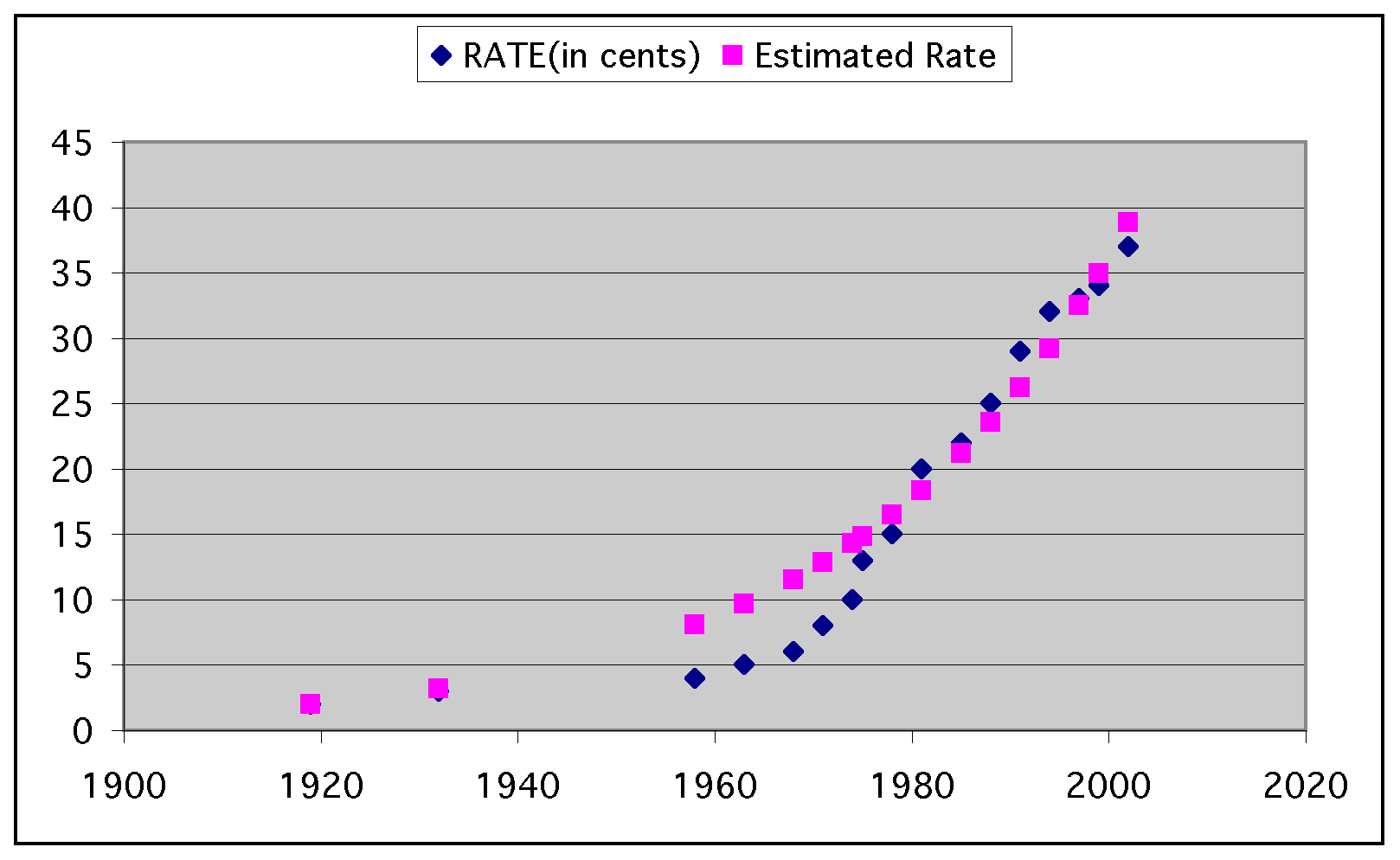
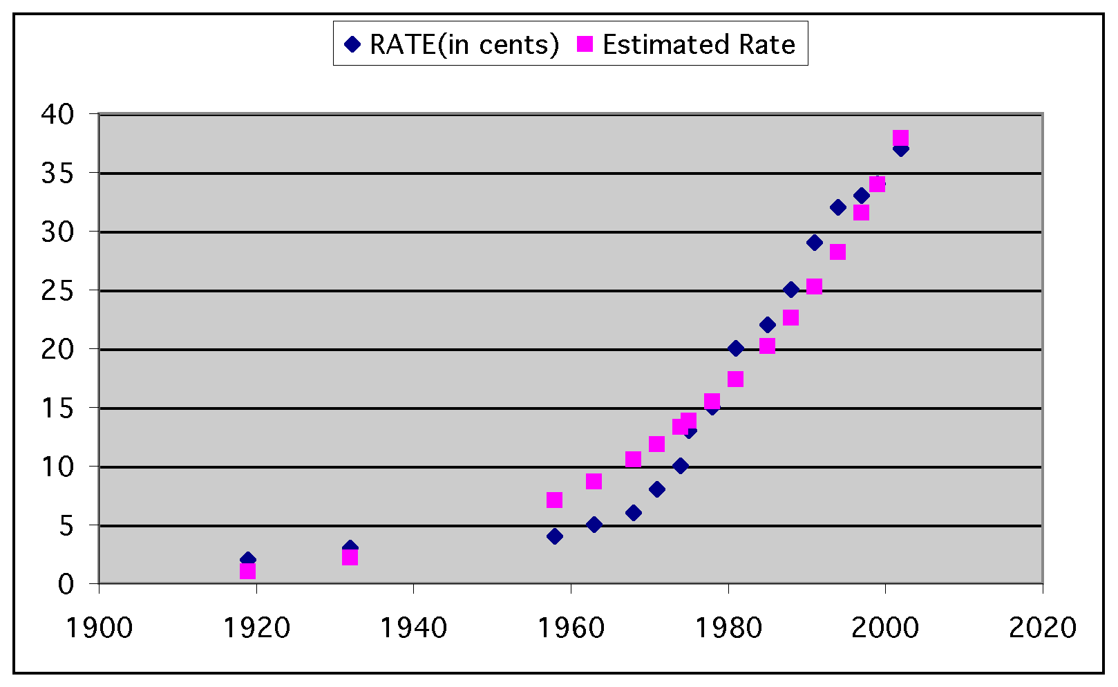
Now we can graph the estimated rates against the observed rates and see how they compare. We can also see the difference created by subracting one from the function:
2*1.2^((current year-1919)/5.1)

price = 2*1.2^((current year-1919)/5.1)-1:

How can we use our equation to predict when the cost of a first class postage stamp will reach $1.00?
Our predicion function:
price = 2*1.2^((current year-1919)/5.1)-1.
To find the year when postage will reach $1.00, simply set this function equal to $1.00 and solve for the 'current year' in the equation.
100 = 2*1.2^((current year-1919)/5.1)-1
(100+1)/2=1.2^((current year-1919)/5.1)
ln48.095=((current year-1919)/5.1)ln1.2
Using the ln function, these values can also be calculated in spreadsheet software:
(3.873178)=((current year-1919)/5.1)(0.182322)
21.24=(current year-1919)/5.1
108.34=current year - 1919
1919+108=2027.
From this result, we can predict that the price of first-class stamps will be $1.00 in 2027.
When will the cost be 64 cents?
We can answer this question just as we did above, by setting our equation equal to 64 and solving for the 'current year'.
64= 2*1.2^((current year-1919)/5.1)-1
3.45=((current year-1919)/5.1)(0.182322)
current year=96.68+1919
From this we can conclude that the price of stamps will reach 64 cents in 2015.
When can we expect the next 3-cent increase?
To find the answer to this question, we need to use our equation and set it equal to the current price of stamps plus 3 cents, or 40 cents:
40 = 2*1.2^((current year-1919)/5.1)-1
Using the same methods as above, we find that the next 3-cent increase in the price of first-class stamps will occur in 2002...
If we remove the constant from the function, the 3-cent increase would happen later in 2002, so this would not remedy our faulty forecast for 40-cent stamps. Our review of the total absolute difference between the expected and observed prices indicates that the prediction function selected is the "best-fit" for the entire history of prices of stamps. Obviously there is some adjustment required in the calculation; perhaps the forecast would have been better modeled on recent (within the past 20 years) price increases only.