Parametric Equations
by
Brock F. Miller
From Dr. James Wilson's Web Page:
A parametric curve in the plane is a pair of functions


where the two continuous functions define ordered pairs (x,y).
The two equations are usually called the parametric equations
of a curve. The extent of the curve will depend on the range of
t and your work with parametric
equations should pay close attention the range of t . In many
applications, we think of x and y "varying with time t"
or the angle of rotation that some line makes from an initial
location.
Various graphing technology, such as the TI-81, TI-82, TI-83,
TI-85, TI-86, TI-89, TI- 92, Ohio State Grapher, xFunction, Theorist,
Graphing Calculator 2.1, and Derive, can be readily used with
parametric equations. Try
Graphing Calculator 2.7 or xFunction for what is probably the
friendliest software.
For this investigation
we will be using Graphing Calculator 3.1 to illustrate various
parametric equations. This write-up is intended to familiarize
the reader with parametric equations and what certain parameters
control on certain parametric equations.
Consider
the parametric equation:

for t in the interval
0 < t < 360 degrees
From discussions in class we are familiar
with cosine and sine. Before we start looking at the graphs let's
discuss what we think should happen. We know that cosine and sine
have a range of [-1 , 1]. Therefore since x = cos(t) it would
make sense that the x-values would range from [-1 , 1]. Likewise
for y = sin(t) should tell us that y will range from [-1,1]. Looking
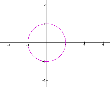
at the graph for this parametric equation.

We see that in fact x-values and y-values
do in fact stay in the range [-1 , 1].
This should be familiar to you as the Unit
Circle.
Now let's investigate what various parameters
can control on this equation.
Consider:

Where a and b are any real number not equal
to 0. (Note to reader: a and b can in fact equal zero but for
the purpose of anything interesting we will not consider these
cases.)
We will consider three cases for a and b:
CASE I: a = b,
CASE II: a > b, and
CASE III: a < b.
CASE I: a = b
We saw in our previous example of the unit
circle that in fact we looked at one case when a = b. For that
example a = b = 1. Now let's look at other values.


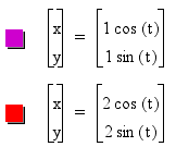
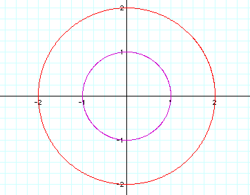
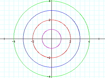
We should notice that the centers of our two
circles remains the the origin but when we change parameters a
and b to a value of 2 we obtain a circle with a radius of 2. It
would make sense that this case when a = b we will obtain a circle
with a radius of a or b.
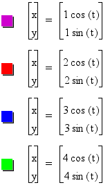
Looking at various a = b cases:


In conclusion when a = b in this particular
equation we obtain a circle centered at the origin with a radius
of a = b.
CASE II: a > b
From our talk about domain and range earlier
with our first look at these parametric equations we see that
the values of a and b control the range of values for x and y.
In fact in terms of (x,y) the a controls the domain and the b
controls the range.
Consider:

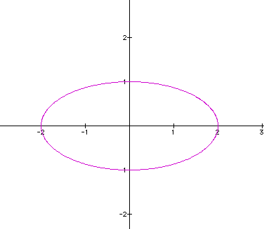
Analyzing this equation should tell us that
x should be in the interval [-2 , 2] and the y should be in the
interval [-1 , 1]. With that in mind we should not obtain a circle
as a curve.

Just as our assumptions have held true. We
see an ellipse. The greater value of a actually stretched the
circle out on unit in the horizontal direction. If we continue
to let a grow we should just obtain a larger "stretch"
of the ellipse.


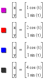
We notice in the range of a values 1,2,3,
and 4, we start with the unit circle and with each growing value
of a we see a stretch in each horizontal direction by a magnitude
of a.
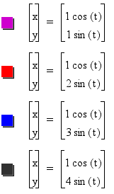
CASE III: a < b
From Case II, we concluded that when a >
b we get an ellipse that stretches horizontally along the x-axis
by a magnitude of "a". Now if we let b become larger
we might see an ellipse that stretches in the vertical direction
by a magnitude of b.
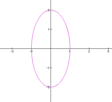
Consider:

Clearly, x will be in the interval [-1 , 1]
and y will be in the interval [-2 , 2].
Graphically:

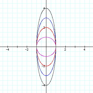
Which is indeed what we expected. Looking
at different values of b we can see this idea of a vertical stretch
to remain constant.


The graphs hold true to our assumption.
This family of parametric equations is interesting and much visually
nicer to look at in terms of equations then that of the traditional
y = equation. From this there are other questions to consider:
I) How will we move the center of these curves
horizontally?
II) How will move the center of these curves
vertically?
III) Will a period change of these two functions
cause any change?
With an adequate graphing program or calculators
these ideas can easily be investigated. If you have any questions
or comments please email me from my home page.


