Although I have used Theorist for several different Write-Ups, I think you can always learn something new about software. Usually, the software provides short cuts for creating different functions. To explore polar equations, Theorist allows you to enter the equation with variable coefficients. For instance, look at the equation below:

I can manipulate each variable one at a time without having to make a new notebook and retype the equation.

I would first like to start this exploration by making all the variable equal to zero except for one. Let's first start this exploration by graphing a = 1 and b,n,c = 0. (r=1)

The equation forms a circle with the radius at one. Now, lets manipulate the graph and try a = 2 and -1.

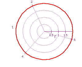
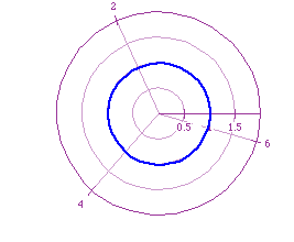
The drawing in red, a = 2 makes the circles radius equal to 2, while the blue circle, a = -1, makes the circles radius equal to 1. So now we can make a hypothesis, when the equation, r = a, will make a circle with radius equal to the absolute value of a.

Next, lets explore r = b cos (0) for different values of b. The first equation is r = cos (0).

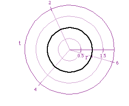
Again, notice the equation leads us to a circle with radius 1. If I graphed different values of b, the graph would be a circle with radius equal to the absolute values of b. This is exactly what graphing a looked like. Now, would if I said r = a + b cos (0) and varied a and b. What would this graph look like? Let's first try r = 1 + cost (0).

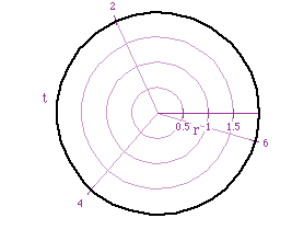
Something interesting happens, the radius is now 2 (a + b). We can hypothesize about other values of a and b. Below is a graph of r = 1 + 2 cos (0) and r = .5 + .5 cos (0).

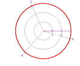
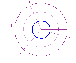
After graphing the polar equations, our conjecture still holds true. We have not found a counterexample to disprove the conjecture. The equation r = a + b cos (0) will graph a circle with the absolute value of (a + b). Try to graph the equation r = -.5 + .5 cos (0), you should get a point.

To continue our exploration, lets add the variable n into the equation r = a + b cos (n t). The graph below is a = 1, b = 1, and n =1.

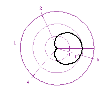
Finally, we have a graph that is not a circle. To continue the exploration, let's look at the different values of n. Let's start with 2 and .5.

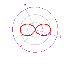
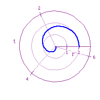
Using these two coefficents tells me nothing. I will animate the variable n and see what the graph does between t = 0 to 2 pi. The graph starts out as a circle and then goes to the blue example above. Eventually, the graph forms 2 to 5 pedals. After the 5 pedals are formed, the graph starts over, with a circle.

Now, I would like to animate the a coefficient. First, I will try a = 0 and n = into the equation r = a + b cos (nt )

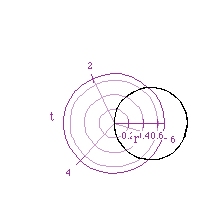
When I animate a, the graph starts out like above. Then, moves to a circle with a loop in it. Then, the figure gets larger and larger until it goes off the axis. Of course, this repeats. I am going to animate b to see how the graph changes. Of course the graph starts out with a circle, when animated, the graph always goes through (0,0) and the circle continues to get larger and larger. If we animate n, the graph "grows" pedals until it grows it's maximum number of pedals below. The equation is r = 1 + 1 cos (2p t).

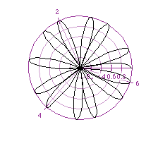
The picture formed 12.5 pedals.

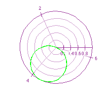
Add a new variable into the equation, r = 1+1 cos( t + c), where t is the parameter. The graph is below and the c value is equal to 1.

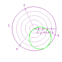
The circle is now translated down. Instead of the radius lying on t = 0 line it now lies below this line. What do you think might happen to the graph if used animation? Just like we suspected, the graph keeps the same shape, but moves arount the polar coordinate. Below is a "snapshot" of what happens to the graph.

This exploration explored how each coefficient independently, changed the original graph.