

It has now become a rather standard exercise,
with availble technology, to construct graphs to consider the
equation
and to overlay several graphs of
for different values of a, b, or c as
the other two are held constant. From these graphs discussion
of the patterns for the roots of
can be followed. For example, if we set
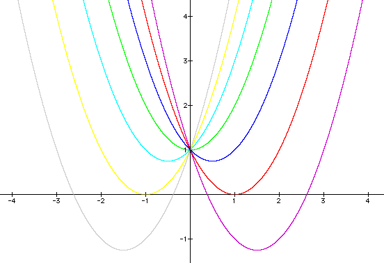
for b = -3, -2, -1, 0, 1, 2, 3, and overlay
the graphs, the following picture is obtained.
Where the graph can be labeled:
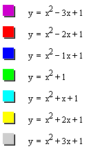
We can discuss the "movement"
of a parabola as b is changed. The parabola always passes through
the same point on the y-axis ( the point (0,1) with this equation).
For b < -2 the parabola will intersect the x-axis in two points
with positive x values (i.e. the original equation will have two
real roots, both positive). For b = -2, the parabola is tangent
to the x-axis and so the original equation has one real and positive
root at the point of tangency. For -2 < b < 2, the parabola
does not intersect the x-axis -- the original equation has no
real roots. Similarly for b = 2 the parabola is tangent to the
x-axis (one real negative root) and for b > 2, the parabola
intersets the x-axis twice to show two negative real roots for
each b.
Now consider the locus of the vertices of the set of parabolas
graphed from
Show that the locus is the parabola
Generalize.
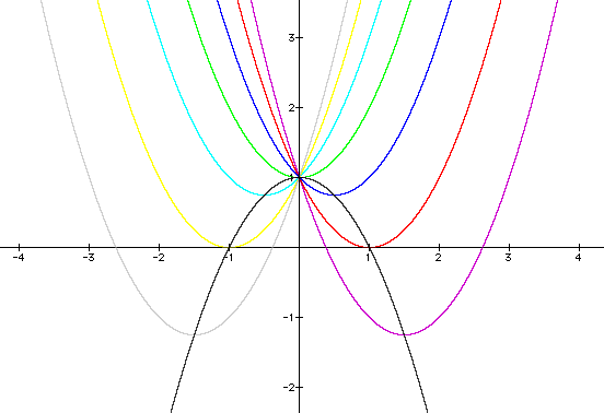
Where the graph can be labeled:
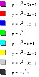
Now lets examine how these graphs change in the varying planes.
Consider the equation
Now we can graph this relationship to examine further:
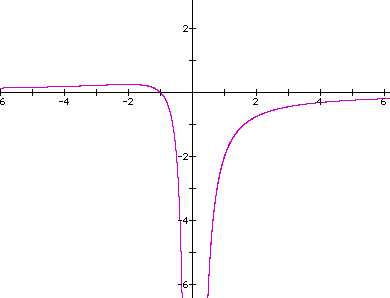
If we now look at a particular value for a, say a=-1, and overlay this graph with the original we add a parallel line at a=-1. This parallel line will give some implication of the roots for the original equation because the intersection(s) in the xa plane will correspond to those roots.
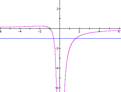
For each value of a that we select, we will get a horizontal line. It can also be seen that when we select a=-1 we get two negative roots of the equation. We can also visualize that when a>0 there will be two negative roots. When a=0 there will be no roots. However when a>.25 there are also no roots. When .25>a>0 there is one root for the equation.
We can also examine what occurs in the
xa plane if we change the equation. When we look at the graph
and vary the variable b from 1 to examine other values the equation
changes in appearance. If we look at the b value from -5 to 5.
We get an equation ![]() where b is changing and the graph looks like:
where b is changing and the graph looks like:
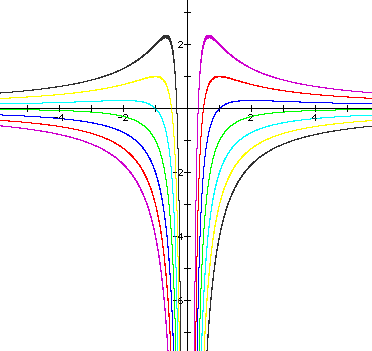
Where the graph can be label as follows:
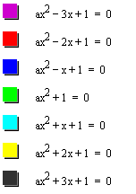
We can also examine what occurs in the
xa plane if we put b back to 1 and change c and vary c for the
values -3 to 3. We get an equation that appears as ![]() and
a graph that looks like:
and
a graph that looks like:
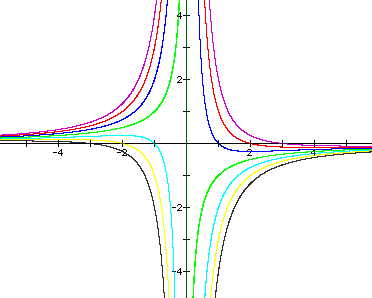
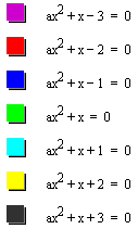
Where the graph can be labeled:
Therefore from the graphs in the xa plane one can see that setting a graph with a specific value for b and c gives a representation of a graph where a is a hyperbola that is approaching .25 as it goes to negative infinity and zero as it approaches positive infinity. The y value of the graph is also approaching negative infinity as x approaches zero. When a is varyed and different values of b are examined the graph moves to a sharper positive value as x approaches zero. but then still drops to negative infinity. When the b value is negative the sharp point is on the right hand side of the graph and when the b value is positive the sharp point is on the left hand side of the graph. When c is varied and b is held constant the value is then smoothed out and the curve forms a more standard hyperbola.
Consider again the equation
Now graph this relation in the xb plane.
We get the following graph.
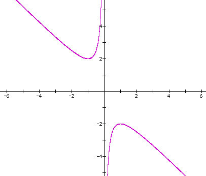
If we take any particular value of b,
say b = 3, and overlay this equation on the graph we add a line
parallel to the x-axis. If it intersects the curve in the xb plane
the intersection points correspond to the roots of the original
equation for that value of b. We have the following graph.
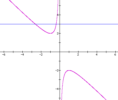
For each value of b we select, we get
a horizontal line. It is clear on a single graph that we get two
negative real roots of the original equation when b > 2, one
negative real root when b = 2, no real roots for -2 < b <
2, One positive real root when b = -2, and two positive real roots
when b < -2.
Now consider the case in the xb plane if we leave b and change
the values of a from -3 to 3. We get an equation that appears
as ![]() and a graph that
looks like:
and a graph that
looks like:
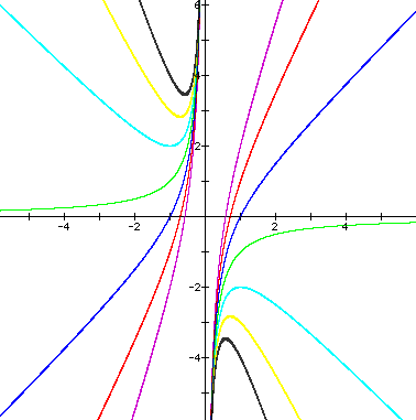
Where the graph is labeled:
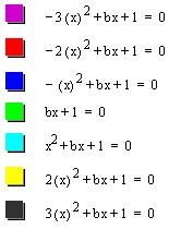
Now lets consider the case where c is
varying from -3 to 3 and a is back to the constant 1. We get an
equation that looks like
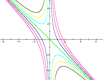
Where the graph can be labeled:
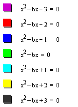
From the graph when the a value was being
changed from -3 to 3, one can see that what is happening is that
the graph loop is spreading out closer to a straight line. This
should make sense from our background in understanding equations.
As we change the coordinate a the graph essentially changes in
the width of the curve. The graphs also appear to be approaching
y values of infinity and negative infinity. However one could
also see that when the a value is negative the curve is more defined,
much like a parabola, and when the curve is positive it is looking
more like a straight line. When the curve is zero, the graph is
a hyperbola also approaching negative and positive infinity with
its x values and based solely in quadrant II and IV. When we move
the a value back to a constant of one, and look at varying the
c value from -3 to 3, then the graph still has a hyperbolic like
shape however there is a defined like at the line that goes through
the origin with a negative one slope. As one can see from the
curve when the c value is negative the curve is approaching the
line and negative infinity getting closer and closer to x=0, and
then is the exact image reflected over the line ![]() and
approaches the line and positive infinity getting closer and closer
to x=0. The positive c values have curves that are only in quadrant
II and IV, just like the a values. These curves approach the line
and x=0.
and
approaches the line and positive infinity getting closer and closer
to x=0. The positive c values have curves that are only in quadrant
II and IV, just like the a values. These curves approach the line
and x=0.
In the following example the equation
is considered. If the equation is graphed
in the xc plane, it is easy to see that the curve will be a parabola.
For each value of c considered, its graph will be a line crossing
the parabola in 0, 1, or 2 points -- the intersections being at
the roots of the orignal equation at that value of c. In the graph,
the graph of c = 1 is shown. The equation
will have two negative roots -- approximately -0.2 and -4.8.
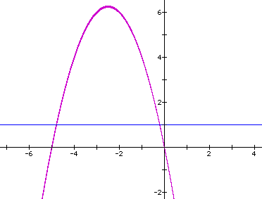
There is one value of c where the equation will have only 1 real root -- at c = 6.25. For c > 6.25 the equation will have no real roots and for c < 6.25 the equation will have two roots, both negative for 0 < c < 6.25, one negative and one 0 when c = 0 and one negative and one positive when c < 0.
Again we can examine how the curve would
change if we were to change our a and b variables. Let us first
consider our a variable. If we look at the equation ![]() in the xc plane when we change the a variable between -3 and 3
we get a graph that appears as:
in the xc plane when we change the a variable between -3 and 3
we get a graph that appears as:
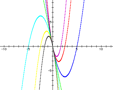
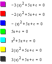
Where the graph can be labeled:
Now if we change a back to the constant
1 and vary b from from -3 to 3 with the black line showing the
original 5 value given for b we get an equation that looks like
![]() with a graph that appears as:
with a graph that appears as:
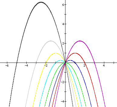
Where the graph is labeled as:
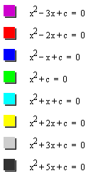
This information found in the xc planeis very interesting. The first graph considered, when a and b were constant, shows a parabola. When the a value is examined and the value is varied from 1 to numbers between -3 and 3, the graph changes in width and also in direction. The direction should be confusing at first because typically when a is a negative number the parabola will be concave down and when the a value is positive the graph will be concave up. In this case however, when a is positive it is concave down and when a is negative it is concave up. This is because of the change in the xc plane. The a value is changed it also varies the width (slope) of the graph. Because a is changing the vertex also changes but the y-intercept is always (0,0) because that is the origin (in XC plane). The case of when a=0 is also interesting because when a=0, the graph is a line. This line is interesting because it seems to be the divider between the two sets of graphs (the positive a's and the negative a's). When examined, one can also see the y-intercept has not been changed and shared the common point, (o,0). When the a value is put back to one and the b value is changed between -3 and 3, the change is seen in the vertex change of the graph. While the concavity has not changes, the vertex seems to be bouncing around. This is because when b is varied, the graph's vertex also changes. The graph will also go through the common point (0,0). The outlier curve is the original constant 5. The graphs vertex seems to be rising and seems to be also increasing in size.
This information is useful because it can be shown that no matter the plane the standard graph is on, a curve can be developed an examined. Before truly understanding parabola and hyperbolic curves, one must understand the differences and the changes made by changing different aspects of the curve. Examination of these curves, should be down more at a high school level. Exploration leads to increased knowledge.