POLAR EQUATIONS

By Shadreck S Chitsonga

The rectangular coordinate system is so popular in mathematics, that it masks the other systems. Most of our students are familiar plotting the points (x,y) in the coordinate plane.

What about polar coordinates? Do students feel comfortable with them? In this write up I will discuss the polar coordinates. I will try to draw parallels with the rectangular coordinate plane.

As usual let us start with something that I think most us are familiar with, yes the rectangular coordinate(Cartesian) plane.

We will make use of the graphing calculator.

Let us plot a few points in the coordinate plane, A (2,4), B(-3,2) C(-2.-4), D(3,-3)

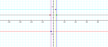
Though trivial, but it is worth noting that each of the plotted points is defined by the intersection of two lines, one parallel to the x-axis and the other parallel to the y-axis.

For example the point B (-3,2) which is the red dot, is the point of intersection between the lines x = -3 and y = 2. All the other points are defined in this way in the rectangular coordinate system.

But is this the only way we can describe the position of a given point in the plane?

Let us consider a point (x, y) in the coordinate plane. Let that point be (4,4). The point is plotted in figure 1.

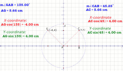
Figure 1

ABC is a right - angled triangle. We know that the point C is defined as (x,y) = (4, 4) in the rectangular coordinate plane. The angle CAB is equal to 45. Let us define the point C with respect to the angle CAB.

We know that sine of an angle is defined as the and that cosine of an angle is

In this case sine angle BAC = BC/AC, we can therefore say that BC =AC x Sine of angle BAC and similarly cosine of BAC = AB/AC which means that AB = AC x Cosine of BAC.

If we look at the expressions AC •cosine (45°) and

AC•sine(45°) , we see that these two are equivalent to the coordinates of point C in the rectangular coordinate plane. Similarly the point G is defined by AG•cosine(135°) and AG • sine(135°).

Now we have a new way of representing points in a plane. In this case we see that AG = AC is the radius of a circle. An angle and a radius therefore define each point.

This coordinate system is defined as the polar coordinate system.

(x,y) in the rectangular coordinate system is equivalent to (r, angle).

In polar coordinates x = r cos q and y = r sin q

Now instead of the rectangular grid we have points defined by the intersection of a circle and a line.

Now it is time to explore a few polar equations. We will investigate graphs for the functions of the form r = a + b cos(kq).

We will first of all consider a situations when a and b are equal and k is an integer.

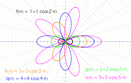
Figure 2

Here we can see that the number of “leaves” for the rose depends on the value of k. For k=2, we have two leaves, k =3 we have 3 leaves. In other words as the number k gets larger and larger, the number of leaves also increases.

The values of a =b determine how big the leaf is, if a and b are increased by a factor m, the leaf is also stretched m times.

In figure 2, compare the black curve and the green curve.

If you look at the polar grid, there is something that you will notice with the five functions plotted.

For example the curve for the function is enclosed in the circle of radius 5+5=10. The same is true with all the other functions. The radius of the circle that encloses the curve is determined by the value of a=b.

If k is an even number then the rose has at least a pair of its leaves lying in the y or x- axis.

If k is odd none of the leaves does that.

If we replace cos() with sin(), we get the following curves:

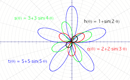
Figure 3

There are a number of observations we can make here:

1. The number of leaves still depends on the value of k.

2. The radius of the circle enclosing the curve still depends on the value of a = b.

3. The quadrant in which the leaves lie depend on the value of k. Consider the cases when k=3 and k=5. With k=3, one of the leaves lies in the negative y-axis, while with k = 5, one of the leaves lies in the positive y-axis.

4. Ignoring the part of the leaf that crosses the x-axis, we see that the number of leaves above the x-axis is always one greater than the number of leaves below the x-axis.(Apart from when k=2)

Now let shift our focus to conic sections. My assumption here is that you are already familiar with the basic shapes of parabola, hyperbola and ellipse.

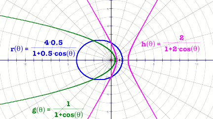
Figure 4

The diagram above shows three different types of curves. For the time being we can say that they look like parabola, hyperbola, and ellipse respectively. Please look at he functions carefully. They are a number of similarities and differences.

For example

1. They are functions involving cos(q).

2. The cosine is in the denominator in all of them.

3. The curve that we think is an ellipse has 0.5 as the coefficient of cos(q) , the one with think is a parabola the coefficient is 1 and the hyperbola, the coefficient is 2. Is there any thing special with these numbers?

If you want more insight, CLICK HERE.