
| This is the write-up of Assignment #3 |
Brian R. Lawler
|
| EMAT 6680 |
12/8/00
|
![]()
and to overlay several graphs of
![]()
for different values of a, b, or c as the other two are held constant. From these graphs discussion of the patterns for the roots of
![]()
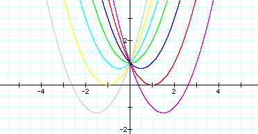
can be followed. For example, if we set ![]() for b = -3, -2, -1, 0, 1, 2, 3, and overlay the graphs, the following
picture is obtained. (Click on the graph itself to download a file for exploration.
Do this on any graph on the page.)
for b = -3, -2, -1, 0, 1, 2, 3, and overlay the graphs, the following
picture is obtained. (Click on the graph itself to download a file for exploration.
Do this on any graph on the page.)
 |
|
We can discuss the "movement" of a parabola as b is changed. The parabola always passes through the same point on the y-axis (the point (0,1) with this equation). For b < -2 the parabola will intersect the x-axis in two points with positive x values (i.e. the original equation will have two real roots, both positive). For b = -2, the parabola is tangent to the x-axis and so the original equation has one real and positive root at the point of tangency. For -2 < b < 2, the parabola does not intersect the x-axis -- the original equation has no real roots. Similarly for b = 2 the parabola is tangent to the x-axis (one real negative root) and for b > 2, the parabola intersects the x-axis twice to show two negative real roots for each b.
Now consider the locus of the vertices of the set of parabolas
graphed from ![]() .
.
See that the locus is the parabola ![]() .
.
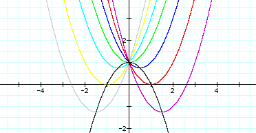 |
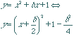
To prove that ![]() is the locus of the vertices of the parabola, consider the set of vertices
of all quadratics of the form
is the locus of the vertices of the parabola, consider the set of vertices
of all quadratics of the form ![]() .
.
| By rewriting in vertex form |
|
||
| the general form of the vertices can be seen to be |
|
||
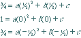
| Substituting 3 values for b will identify 3 particular points. The unique quadratic through those three points can identified with linear algebra. |  |
 |
|
Hence, ![]() passes
through all vertices.
passes
through all vertices.
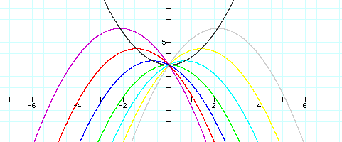
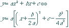
To generalize this hypothesis, observe similar results in quadratics with other a and c coefficients. For example, in the case below, a = -0.7 and c = 3.
 |
|
See that the locus of this family of quadratics can be defined
in general by ![]() .
.
| Again, by rewriting the general quadratic in vertex form |
|
||
| the general form of the vertices can be seen to be |
|
||
Substituting 3 values for b will identify 3 particular
points. The unique quadratic through those three points can be verified to
be![]() with linear algebra.
with linear algebra.
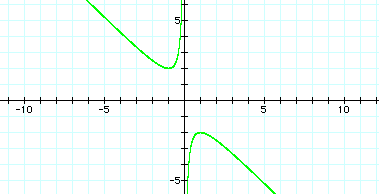
Consider again the equation
![]()
Now graph this relation in the xb plane. We get the following graph.
If we take any particular value of b, say b = 5, and overlay this equation on the graph we add a line parallel to the x-axis. If it intersects the curve in the xb plane the intersection points correspond to the roots of the original equation for that value of b. We have the following graph.
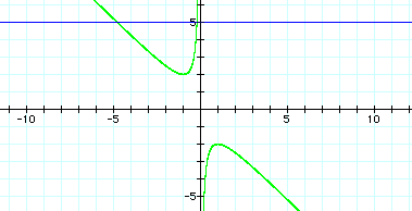
For each value of b we select, we get a horizontal line. It is clear on a single graph that we get two negative real roots of the original equation when b > 2, one negative real root when b = 2, no real roots for -2 < b < 2, one positive real root when b = -2, and two positive real roots when b < -2.
Consider the case when c = - 1 rather than + 1. (In the example below, I had to use the y variable to mimic the b. Otherwise, you will see everything works the same - this is why I left the original equation in green.)
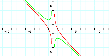 |
|
Again, for each value of b we select, we get a horizontal line. It is clear on a single graph that we get two real roots of the original equation for all values of b . One root will always be positive, and the other negative.
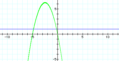
It is possible to consider many values of c all at one time. First, move the c to the other side of the functions. Then, observe a contour plot or a 3D graph to observe the effects of changing c as x and b are free.
![]()
is considered. If the equation is graphed in the xc plane, it is easy to see that the curve will be a parabola. For each value of c considered, its graph will be a line crossing the parabola in 0, 1, or 2 points -- the intersections being at the roots of the original equation at that value of c. In the graph, the graph of c = 1 is shown. The equation
![]()
will have two negative roots -- approximately -0.2 and -4.8. (Again,note that in the example below, I had to use the y variable to mimic the c. Otherwise, you will see everything works the same.)
 |
|
There is one value of c where the equation will have only 1 real root -- at c = 6.25. For c > 6.25 the equation will have no real roots and for c < 6.25 the equation will have two roots, both negative for 0 < c < 6.25, one negative and one 0 when c = 0 and one negative and one positive when c < 0.
Interestingly, varying this value of b while graphing in the xc
plane will yield the same behavior as was seen in the initial problem of graphing
![]() in the
xy plane. We will leave it to the reader to explore and explain this
phenomenon.
in the
xy plane. We will leave it to the reader to explore and explain this
phenomenon.
Also, how about graphing in the xa plane? Happy mathematics!
 |
Comments? Questions? e-mail either of us at: |
Dr. Jim Wilson
|
jwilson@coe.uga.edu |
|
Brian Lawler
|
blawler@coe.uga.edu |
| Last revised: December 28, 2000 |
|
 ,
,
 ,
,