With current available technology,
it has now become a rather standard exercise to construct and
overlay several graphs of ![]() for different values of a,
b, or c while two values are held
constant. From these types of graphs, the patterns for the roots
can be discussed about the following function:
for different values of a,
b, or c while two values are held
constant. From these types of graphs, the patterns for the roots
can be discussed about the following function:
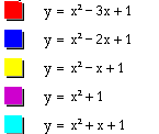
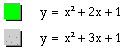
Let's begin examination of the
function ![]() with the values for b set
at b = -3, -2, -1, 0, 1, 2, 3. With the graphs overlayed,
the following picture is obtained.
with the values for b set
at b = -3, -2, -1, 0, 1, 2, 3. With the graphs overlayed,
the following picture is obtained.
We can discuss the "movement" of a parabola as b is changed. The parabola always passes through the same point on the y-axis ( the point (0,1) with this equation). For b < -2 the parabola will intersect the x-axis in two points with positive x values (i.e. the original equation will have two real roots, both positive). For b = -2, the parabola is tangent to the x-axis and so the original equation has one real and positive root at the point of tangency. The real and positive root is 1 since (x-1)(x-1) are the factors of the parabola function when b=-2. For -2 < b < 2, the parabola does not intersect the x-axis, therefore, each corresponding equation doesn't have any real roots. Similarly, for b = 2 the parabola is tangent to the x-axis and has one real negative root. For b > 2, the parabola intersects the x-axis twice to with two negative real roots.
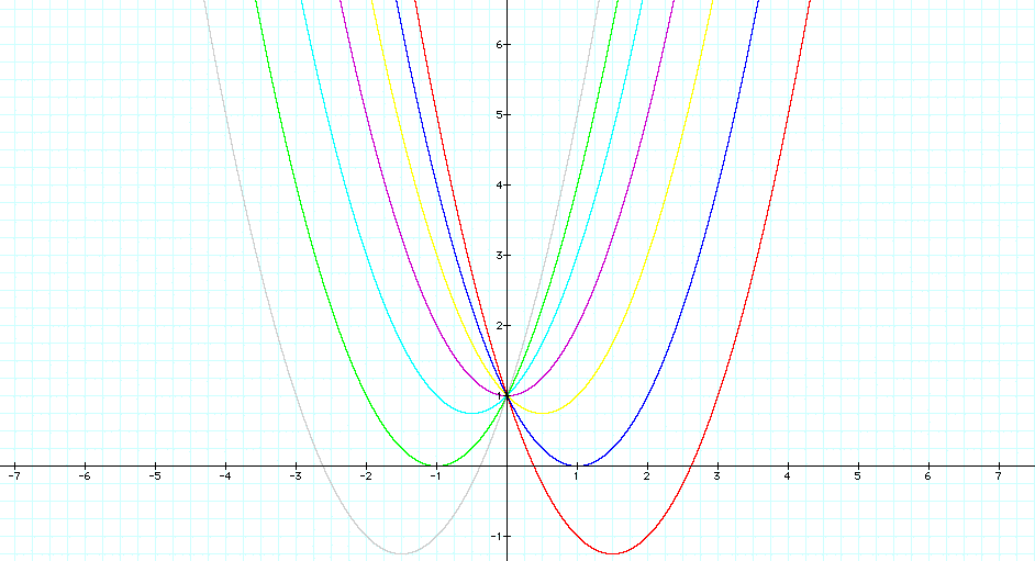
Now consider the locus of the
vertices of the set of parabolas graphed from ![]() .
The locus is the line or surface made up
of all the positions of a point or line satisfying some condition.
For example, the locus of points equidistant from a fixed point
is a circle. The locus is the parabola is
.
The locus is the line or surface made up
of all the positions of a point or line satisfying some condition.
For example, the locus of points equidistant from a fixed point
is a circle. The locus is the parabola is ![]() . For reference, see the graph below of the parabola function
. For reference, see the graph below of the parabola function
![]() for values of b
from -3, -2, -1, 0, 1, 2, 3 along with the locus
function of the set of these parabolas.
for values of b
from -3, -2, -1, 0, 1, 2, 3 along with the locus
function of the set of these parabolas.
Graphs in the xb plane.
Consider again the equation
![]() . Upon graphing this relation in
the xb plane, the following graph is obtained.
. Upon graphing this relation in
the xb plane, the following graph is obtained.
If we take any particular value of b, say b = 3, and overlay this equation on the graph we add a line parallel to the x-axis. If it intersects the curve in the xb plane, the intersection points correspond to the roots of the original equation for that value of b. We have the following graph.
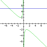
For each value of b we select, we get a horizontal line. It is clear on a single graph that we get two negative real roots of the original equation when b > 2 and one negative real root when b = 2. We don't get any real roots for -2 < b < 2. However, there is one positive real root when b = -2 and two positive real roots when b < -2.
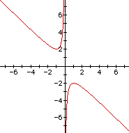
Consider the case when c = -
1 rather than + 1.
Graphs in the xc plane
In the following example, the
equation ![]() is considered. If the equation
is graphed in the xc plane, it is easy to see that
the curve will be a parabola. For each value of c
considered, the graph will be a line crossing the parabola in
0, 1, or 2 points with the intersections being at the roots of
the original equation. In the graph below, the graph of c
= 1 is shown.
is considered. If the equation
is graphed in the xc plane, it is easy to see that
the curve will be a parabola. For each value of c
considered, the graph will be a line crossing the parabola in
0, 1, or 2 points with the intersections being at the roots of
the original equation. In the graph below, the graph of c
= 1 is shown.
The equation ![]() will
have two negative roots at approximately -0.2 and -4.8.
will
have two negative roots at approximately -0.2 and -4.8.
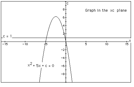
There is one value of c where the equation will have only 1 real root. This value is at c = 6.25. For c > 6.25, the equation will not have any real roots and for c < 6.25, the equation will have two roots. The real roots will both be negative for 0 < c < 6.25 and there will be one negative root and one root at 0 when c = 0. Finally, there will be one negative root and one positive root when c < 0.
In this article, various ways
to examine ![]() have been explored. Further investigation can
be implemented through math technology tools such as Graphing
Calculator which was the program of choice for this article.
have been explored. Further investigation can
be implemented through math technology tools such as Graphing
Calculator which was the program of choice for this article.