Learning and experimenting with
Polar Equations
"Smelling the Mathematical
Roses"
In investigating certain curves it can be more convenient to locate a
point by means of its polar coordinates. The polar coordinates give its
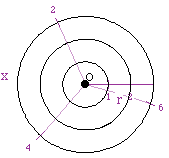 position relative to a fixed reference point O (the pole) and to a given
ray (the polar axis) beginning at O. The diagram to the left shows a standard
polar graph. Points are placed on this graph using a coordinate system where
(r,x) is the ordered pair that represents r = the distance from the origin
and x = the angle measured counterclockwise from the x axis and terminal
arm. An example would be (3,0) this would place a point on the third
ring out at an angle of 0. Another example would be (1,pi/2), this would
place a point directly above the origin on the first ring.
position relative to a fixed reference point O (the pole) and to a given
ray (the polar axis) beginning at O. The diagram to the left shows a standard
polar graph. Points are placed on this graph using a coordinate system where
(r,x) is the ordered pair that represents r = the distance from the origin
and x = the angle measured counterclockwise from the x axis and terminal
arm. An example would be (3,0) this would place a point on the third
ring out at an angle of 0. Another example would be (1,pi/2), this would
place a point directly above the origin on the first ring.
Equations in polar form are relationships between r and x. A few examples
would be r = 3, or r = 3 cos(x) or r = 1 + 3 sin(2x).... These types of
relationships seem to work out nicely in the polar plane because of the
their heavy reliance on angles and radian measure. Below are a few basic
examples of equations in polar form and their resulting graph.
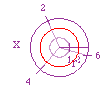
| r = 2 - all points that are a distance of 2 from the pole. |
r = 2 sin(x) - a circle formed with a diameter of 2 |
r = 2 cos(x) - a circle formed with a diameter of 2 |
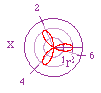
r = 2 cos(3x) - a 3 pedal shape is form that extends out to max. |
 |
 |
 |
 |
| for all values of x, r = 2 thus the circle. |
r = 0 when x = 0, thus the orientation |
r = 1 when x = 0, thus the orientation |
value of r = 2. |
Smelling the Roses of Mathematics
To investigate the "n- leaf roses" I will be looking at the
equation r = a + b cos(kx) where r = the distance from the pole
and x = the angle as it varies from 0 to 2 pi. a, b,
and k are variables that I will at some times hold constant while
at other times, manipulate depending on the circumstance which is to be
developed. Before we can looking at how a graph changes with respect to
our manipulations we must first understand the standard form of the graph.
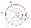
| r = 0 + 1cos(x) - a circle formed with a diameter of 1 |
r = 0 + 3cos(x) - a circle formed with a diameter of 2 |
r = 1 + 1cos(x) - a circle formed with a diameter of 1 |
r = 2 + 1cos(x) - a circle formed with a diameter of 1 |
 |
 |
 |
 |
| As discussed earlier a right orientated circle appears with this equation.
As b variable is manipulated we see the size of the the circle increasing
by that factor. This is because the max. value of cos(x) = 1, thus 3*1 =
3 and the cos(pi/2) value = 0, thus 0*1 = 0. |
(up left) A cardioid is formed from this equation.
Notice the max. value is 2 = 1 + 1 (cos(0)) and the min. value is 0 = 1
- 1 (cos(pi)). (up right) Hopefully you can
now extrapolate why the cardioid has taken on this shape. |
Some general finding that I will not investigate here concerning r =
a + bcos(kx) are:
- if a = b, a general shape is created depending on the other
variables but as a and b are increased or decreased a concentric
similar shape is created about it. Altering a and b by a
constant is the same as multiplying the whole equation by a constant c,
r = c(a + bcos(kx)) thus the natural alteration to its shape.
- if b approaches zero we see the shape approach the shape of
a circle. It would not be a circle until b = 0 because then the
equation would simplify to r = a which is the polar equation form
of a circle.
- if our equation would be r = a + bsin(kx) we would see an orientation
shift because of the nature of the function but the resulting shapes, circles,
cardioids, lemniscate....all appear in a similar fashion.
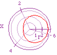
Roses are
created by manipulating the k variable in the equation r = a +
b cos(kx)
- r = 1 + 1cos(2x) blue
- r = 3 + 3cos(2x) red
|
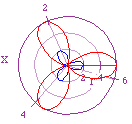
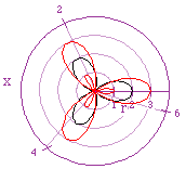
- r = 1 + 1cos(3x) blue
- r = 3 + 3cos(3x) red
|
- r = 1 + 1cos(8x) blue
- r = 3 + 3cos(8x) red
|
 |
 |
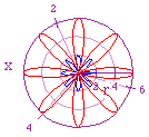 |
| I'm not going to go over why the max and min values occurred, hopefully
that has been understand previously. The number of "leaves" is
what becomes interesting, as k increases we see a direct relationship
with the number of leaves formed. It is also interesting to notice the orientation
difference between an even k and the odd k's. An even k
value can have many axises of symmetry but x = pi/2 (y axis) will always
be one of them whereas for an odd k, x = pi/2 (y axis) will never
be an axis of symmetry as long as k > 1. |
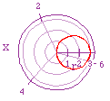
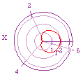
Holding b = 1 and k =3 & 6 while increasing
a, in other words a > b
- r = 1 + 1cos(3x) black
- r = 2 + 1cos(3x) red
- r = 3 + 1cos(3x) green
- r = 4 + 1 cos(3x) blue
|
- r = 1 + 1cos(6x) black
- r = 2 + 1cos(6x) red
- r = 3 + 1cos(6x) green
- r = 4 + 1cos(6x) blue
|
 |
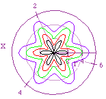 |
This 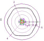 reminds me of Spiro-graph (a great toy). Notice the concentric
nature of these shapes. The max and min values hold true to form in that
cosine restricts the value to be a +- 1. As the difference between
a and b increase where a > b, we see an expansion
from the pole. It is interesting to think about what kind of shape that
would be formed if we continued to increase a. The diagram to the
left shows what the polar equation r = 20 + 1cos(6x) looks like.
It seems to gain much of the shape of a regular hexagon. This does not mean
that it creates a regular hexagon as a approaches infinity but simply that
curve looks like one a this stage. What do you think the shape would be
as a approaches infinity? reminds me of Spiro-graph (a great toy). Notice the concentric
nature of these shapes. The max and min values hold true to form in that
cosine restricts the value to be a +- 1. As the difference between
a and b increase where a > b, we see an expansion
from the pole. It is interesting to think about what kind of shape that
would be formed if we continued to increase a. The diagram to the
left shows what the polar equation r = 20 + 1cos(6x) looks like.
It seems to gain much of the shape of a regular hexagon. This does not mean
that it creates a regular hexagon as a approaches infinity but simply that
curve looks like one a this stage. What do you think the shape would be
as a approaches infinity? |
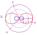
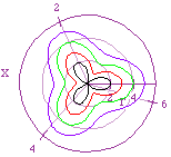
Holding a = 1 and k = 3 while increasing b,
in other words b > a
- r = 1 + 1cos(4x) black
- r = 1 + 2cos(4x) red
|
- r = 1 + 3cos(3x) green
- r = 1 + 5cos(3x) blue
|
 |
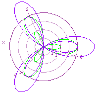 |
| This relationship between a and b create a double leafing
effect. The symmetry of these 3 leaf flowers is quite beautiful. I will
stop my investigation here, although there is much more to discover and
explore. |
The End!!