Final Project by Dorothy Evans

A. Bouncing Barney

Barney is in the triangular room shown here. He walks from a point on BC parallel to AC. When he reaches AB, he turns and walks parallel to BC. When he reaches AC, he turns and walks parallel to AB. Prove that Barney will eventually return to his starting point. How many times will Barney reach a wall before returning to his starting point? Explore and discuss for various starting points on line BC, including points exterior to segment BC. Discuss and prove any mathematical conjectures you find in the situation.

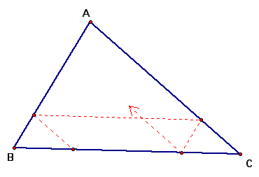
To begin this investigation I created a model of this challenge in GSP.

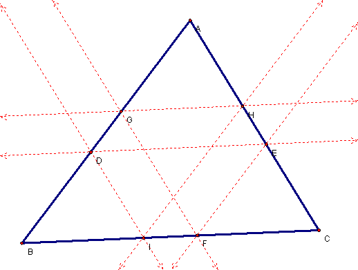
After manipulating the construction it’s intuitively evident that there are only 2 different cases in terms of the number of turns Barney will make before ending at his starting point. In the first case Barney is on the segment BC and is at the midpoint between point B and C. In this case Barney will make only 2 turns (see below) before ending at his starting position.

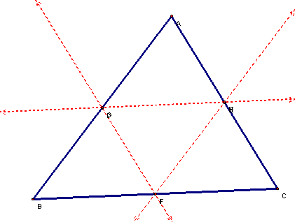
This is because when starting from the midpoint between point B and C and moving parallel to segment AC Barney will end at the midpoint of segment AB. Then moving towards segment AC from the midpoint of AB and parallel to BC Barney will end at the midpoint of AC. Barney’s final turn from the midpoint of AC parallel to AB will put his final destination at the midpoint of BC.

There are multiple ways to prove this but essentially we know that if a line is parallel to one side of a triangle the line divides the triangle into a similar triangle to the entire triangle. Also the sides of the triangle will be proportional. In this case since we started at the midpoints all the parallel lines will end at midpoints and the final result is 4 similar triangles.

The other case is where Barney starts at a point between B and C that is not the midpoint. This point can be on either side of the midpoint.

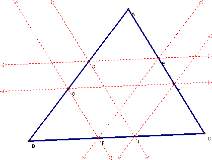
In this case Barney would make 5 turns before returning to his original point on the segment BC. This is also because of similar triangles and the corresponding proportionality that results from the relationship between a parallel line to one side of a triangle. However in this case since the proportions are not ½ the resulting turns are increased because Barney must travel the first proportion and then the reciprocal of that proportion again.

For example, let’s say Barney is 1/3 of the way between B and C (the 1/3 being closer to B). Barney will end up a proportion of 1/3 between B and A (closer to B) when he moves parallel to AC. Then when he lands between A and C he will be 1/3 of the way between A and C (closer to C). Then when he turns toward BC he will be 1/3 of the way between B and C except closer to C ( or 2/3 if measuring closer to B). Then he turns towards AB and lands 1/3 of the way between A and B (closer to A) and turns and lands 1/3 of the way between A and C closer to A this time. Finally on his final turn he is back at his original point 1/3 of the way between B and C.

To explore on your own in GSP click here.

B. Multiple Solutions

Find as many solutions as possible for A, B, and C that satisfy both equations:

ABC = 4

3A + 2B - C = 3.

What observations can you make about your results?

My first step in this is to explore the equations in a 3 dimensional plane. Since this is 2 equations with 3 unknowns the possible solutions are the intersection of the 2 figures.

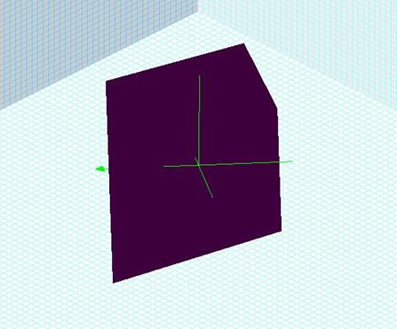
Here is the first equation ABC =4 in the A-B-C plane	Here is the second equation 3A+2B-C = 3

Now let’s put them together

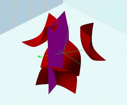
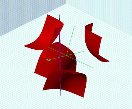
As you can see from these two perspectives of the two figures the graphs intersect resulting in multiple solutions.

Algebraically we can find the solution set by solving for one variable and plugging that variable into the other equation to get our solution set.

I chose to solve for c in the second equation getting C=3A+2B-3. Then I plugged C into the 1^st equation

ABC=4

AB(3A+2B-3)=4

Now we can graph this equation in the A-B plane to visualize the graph of the solution set.

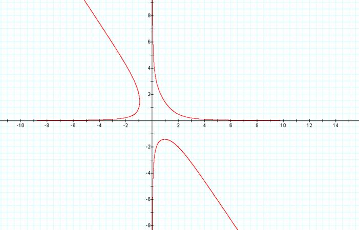
Next we expand the equation to see if we can solve for one of the variables.

Now we can utilize the quadratic equation to solve for A

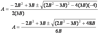
To see the actual values of A given B we utilize a spreadsheet to estimate our solution sets.

One pitfall in spreadsheets that I noticed was that Excel spreadsheets make some assumptions regarding the entered equations.

I found it easier to break up the equation into columns and calculate from there.

First we look at the values of A given integer valued of B for .

A	B+	C+	B-	C-	-b	SQRT	2a
-6	0.031843	-20.9363	10.46816	-0.06369	-126	125.2358	-24
-5	0.044666	-17.9107	8.955334	-0.08933	-90	89.10668	-20
-4	0.06727	-14.8655	7.43273	-0.13454	-60	58.92368	-16
-3	0.113249	-11.7735	5.886751	-0.2265	-36	34.64102	-12
-2	0.234436	-8.53113	4.265564	-0.46887	-18	16.12452	-8
-1	1	-4	2	-2	-6	2	-4
1	1.414214	2.828427	-1.41421	-2.82843	0	5.656854	4
2	0.5	4	-2	-1	-6	10	8
3	0.207825	6.41565	-3.20783	-0.41565	-18	20.4939	12
4	0.108495	9.216991	-4.6085	-0.21699	-36	37.73592	16
5	0.065942	12.13188	-6.06594	-0.13188	-60	61.31884	20
6	0.044184	15.08837	-7.54418	-0.08837	-90	91.06042	24

The first column are the values of A,

the second and 4^th column are the values of B, and

the 3^rd and 5^th column are the values of C.

Notice in columns 7, 8, and 9 that I broke the quadratic equation into 3 parts for my calculations.

This was useful for the reason mentioned above and also to note the relationship between A and each part of the quadratic equation. Do you notice any relationship between the 3 parts and the solutions for B and C? How could we find rational solutions?

I also performed this same calculation for B given A for the integers from -6 to 6.

Then I expanded my calculations to search for solution from -6 to 6 with a step of .1 (i.e A=5.9, 5.8, 5.7 etc)

I completed this for both A given B and B given A.

To see these calculations in EXCEL click here.

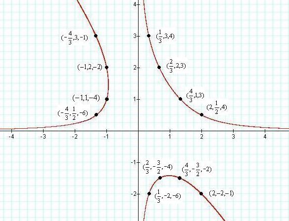
All in all I found 12 real rational solutions; this is not necessarily a comprehensive list. These are

C. Stamp Problem

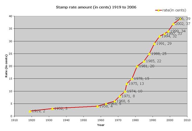
While working out the original Stamp Problem in assignment 12 I noticed that the data was not up to date so I took it upon myself to add the data and compare and contrast the two sets of data. To see my original exploration in assignment 12 click here.

The first few questions are relatively simple to evaluate.

Based on the analysis the cost of a first class postage stamp should reach $1.00 in 2033 and the cost will be 74 cents in 2025.

How soon we should expect the next increase is a totally different analysis. This would require looking at the trend in the increases. There are a few assumptions we will work under. One of these is that the increase will be in integer cents so the increase will have to be more than 1 cent and be an integer increase of 1 or more cents.

Theoretically the next years increase would be 1.4 cents based on the previous model if the decision was made to increase postage next year.

For further analysis on the frequency of increase and the amount of increase I calculated and plotted this data in Excel.

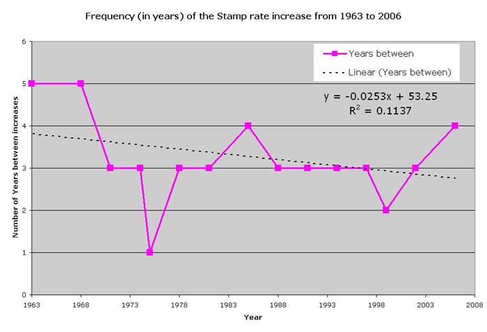
Here (below) we see the frequency in years of each increase. I attempted to model the entire data set but due to the extreme variations between 1919 – 1968 and 1963 – 2006 I chose to eliminate the years from 1919 to 1958 and use a linear model. Based on this data we have a reduction in the frequency of the rate increases over these years. Based on the linear model our next rate increase will be in roughly 2½ years from the last increase in 2006.

To estimate the amount of the increase the following chart was created in Excel.

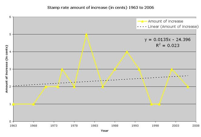
As you can see from this chart the amount of increase is increasing at a steady rate.

Based on this rate and the number of years between increases I would estimate the next increase to be 2 cents in 2 years.

My next best guess would be 3 cents in 3 years.

I guess we’ll see. To see my source data and charts click here.

In 1996, the analysis of stamp data historically seemed to show that the postage doubled every 10 years approximately. The cost in 2006 would seem to argue that pattern is not longer valid. Is there evidence to show a change in the growth pattern? Or, was the ‘doubles every ten years’ just a bad model?

In my evaluation of this model I looked at the increase every ten years. The years that seem to best fit this model are the years from 1963 to 1985. Both the years before 1963 and after 1985 have a much lesser increase. I wouldn’t say it was a bad model, but that the rate increase in 1985 was not twice that of 1975. The increase in 1985 was 2 cents. It would have to have been 4 cents higher for the rate to have doubled since 1975. Also in 1988 the rate increase was 3 cents and it would have to have been an increase of 8 cents to follow this model. In 1991 the increase was 4 cents and it would have had to have been 11 more cents to be double the rate in 1981. It seems to me by 1994 this model should have been retired as an old model that was not useful for the most current data.