
You are the quality control engineer for the Sunshine Sugar Factory. The factory produces processed sugar for various customers who then use the sugar in their manufacturing processes. There are three sugar processing lines, Line Alpha, Line Beta, and Line Gamma. Sunshine has many customers, but there are three major clients whose manufacturing needs are very important to the company. Charlie's Chocolates needs sugar to make chocolate bars, Kathy's Koolers uses sugar to make sweetened beverages, and Patrick's Pie Patch puts sugar into its different pies. Each customer requires different sweetness specifications for the products they will produce from the sugar, and each customer requires approximately 60% of the capacity of one of the processing lines. Based on the customers' sweetness requirements and the quality data for sweetness of the sugar coming from each of the processing lines, you must decide which processing line to allocate to the sugar production for each of the major customers. The quality data for sweetness from each of the processing lines can be found by clicking here, and the individual customer requirements can be found by clicking here.
Charlie's Chocolates wants to determine the weight to put on the label for their new Nutty Swirl candy bar (a chocolate and peanut butter swirled candy bar). One of Charlie's assistants, Lucy, decides to weigh thirty candy bars to get an idea of the appropriate weight for the label. Based on the weights that she finds, discuss with your groups how you would label the candy bars. Click here to see Lucy's data.
Following the group discussion, each group should share their ideas and the teacher should discuss the concepts of mean, median and mode.
There are many situations when we are faced with data. This can be data that we gather from experiments, simulations, or surveys. Or it might be data that is presented in some format from another source. When facing this data, statistics provide a means to examine the data and make some inferences from it. When dealing with any quantitative variable, the distribution of data can be described in terms of shape, center, and spread. We begin our examination of data by talking about measures of central tendency.
Mean
The most common measure of center is the arithmetic average, known as the mean. The mean of a set of data can be found by adding all the values and dividing by the total number of values in the set. If the n values in the set are x1, x2, …, xn, then the mean can be represented as:
 or
or 
Median
Another frequently used measure of central tendency is the median, which is the midpoint of the distribution of data. To find the median, the data should be arranged in order of size from samllest to largest.
If the number of values in the data set is odd, then the median is the data point at the midpoint of the ordered list. For example, if there are 13 data points in the distribution, the median is the 7th data point when all the data is listed in increasing order.
If the number of values in the data set is even, then the median is the mean of the two data points at the midpoint of the distribution. For example, if there are 14 data points in the distribution, then the median is the arithmetic average of the 7th data point and the 8th data point when all the data is listed in increasing order.
Mode
The mode is another measure of central tendency that is more applicable when data is categorical instead of numerical. The mode is the value of the data point that occurs most frequently in the distribution. If there are no repeated values in a set of data points, then there is no mode. If there is more than one value in the data set that is repeated an equal number of times (for instance there are 5 occurrences of the value 4 and 5 occurrences of the value 6 in a data set), then there is more than one mode. For the example mentioned, if 5 occurrences was the most for any specific value, then both 4 and 6 are modes of the data set.
The teacher should demonstrate these concepts using multiple data sets.
Extension Problems
Joe and Janice decided to come up with their own weight for the Nutty Swirl bar, and so they set out to weigh a sample of candy bars. They can't get to the precision scale that Lucy used, so they use two scales that were on the production line. These scales don't measure to the same accuracy that Lucy's scale did, and occasionally they get some readings that seem to be a little off. Using Joe and Janice's data (in spreadsheet with Lucy's data), how would you label the Nutty Swirl bar and why?
Another helpful worker named Larry also wanted to contribute to the effort and decided to weigh his own samples using one of the scales from the production line. Unbeknownst to Larry, Susan the Sneak played a practical joke on him and slipped some extra weight onto the scale while he was weighing his samples. Knowing that some portion of the sample data will have weights that are too high, how could you use Larry's data to label the Nutty Swirl bar? (Note: Larry' data is also in the spreadsheet with Lucy's data)
Carl really likes to drink Strawberry Blast, a fruity drink that comes from a mix made by Kathy's Koolers. He has three different pitchers he uses to mix up Strawberry Blast. Each of the pitchers has a slightly different volume and is shaped differently. Carl has noticed that the strength of his Strawberry Blast varies each time he mixes it, and that the amount of difference between weaker batches and stronger batches varies amongst the three pitchers. Each of Carl's pitchers is cylindrical, but the shape of the base of the cylinder is different. Click here to see the bases of Carl's three pitchers with their dimensions. He has decided that the difference in strength is due to changes in the amount of water added to the Koolers mix to form the Strawberry Blast. Since there are no marks on the pitchers for Carl to guage where he fills the water for the mixture, he decides to measure the height of the liquid in each pitcher whenever he mixes a batch. Because he knows the pitchers are different, he separates his height measurements for each pitcher. Click here to get Carl's height data.
What types of trends do you see in Carl's data? (This should be a topic for group discussion, either in student groups or with the class as a whole.)
In Lesson 1 we discussed measures of central tendency used for describing the center of different data sets. Now we will talk about the spread of the data within a set. The range of the data set can be described as the difference between the minimum value and the maximum value within the set. The spread of the data refers the distance that the majority of the data is from the mean.
For each of the following measures of spread, the term deviation refers to the difference between a data point in the set and the mean of the set.
Mean Absolute Deviation
One method of determining spread is the mean absolute deviation (MAD), which is the average of the absolute values of all the deviations. If the n values in the set are x1, x2, …, xn, then the mean absolute deviation can be represented as:
 where
where 
Variance (s2)
The variance of a data set is determined by averaging the squares of the deviations. There are two formulas for the variance of a data set. One formula is used when the entire population of data is known, and the other is used when there is only a sample of data that represents the population. This second formula for sample variance is the formula most often needed.
Variance for entire population:

Variance for sample population:

Standard Deviation (s)
The standard deviation is the most common measure of spread for describing data sets. It is calculated as the square root of the variance.
Standard deviation for entire population:

Standard deviation for sample population:

The teacher should demonstrate these concepts using multiple data sets.
Extension Problems
How could you use these characteristics to describe Carl's data for each pitcher?
Why would Carl observe a difference in the strength variation of each pitcher if the deviations of height measurements for each pitcher are similar?
Can you think of another type of data that Carl could generate for his pitchers? (the class discussion at this point should lead to analyzing the volume of the pitchers)
How would you describe the characteristics of this data?
Patrick needs sugar for his pies, but he also needs fruit. Edith is in charge of purchasing the fruit, and she is trying to determine how many blueberries to order to maintain the production schedule for Patrick's blueberry pies. She decides to simulate how many blueberries it will take to fill up a single pie shell. She takes one of the pie containers used on the production line and counts how many blueberries it takes to fill it. To make sure she counted correctly, she tries this again and finds that she gets a different number. Frustrated, she repeats the procedure and comes up with a third number. What's going on?
Divide the class into groups of two and use marbles to simulate blueberries. Have each group fill a pie plate five times, then remove the marbles and record many marbles it took to fill the container. (NOTE: the students should be instructed to always fill the pie plate first and then count the marbles they have used to fill it, this way they can't "force" the data to look the same each time, providing a more randomized sample) The data from all the groups should then be compiled and organized using a frequency graph.
How would you describe this shape?
Would you expect to find that a pie plate was filled with x or y number of marbles (pick x and y to be far below and far above the mean)?
Click here to see some examples of different distributions.
The Normal Distribution
We've talked about the center and the spread of the data set, now what about the shape? When data is graphed in the form of a histogram, a curve can be used to approximate the shape formed by the bars in the frequency graph. The normal distribution is one that has a single peak centered about the mean of the data set, it is symmetric about the mean, and the curve approaches zero on either side of the mean, creating a shape that is often called the "bell-shaped" curve.
The normal distribution was identified by a de Moivre, a French mathematician, who used it to make calculations for gamblers. While the distribution is applicable to several situations that are of interest to gamblers, it is also applicable to many other situations. One of these that is of particular interest is measurement variation.
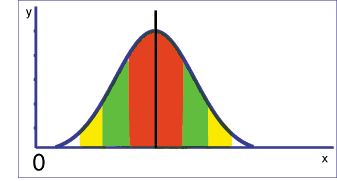
There are some interesting relationships between the normal distribution and standard deviation. Whenever a set of data is normally distributed, approximately 68% of all the results are within one standard deviation of the mean. And approximately 95% of all results are within two standard deviations of the mean. The following diagram is a representation of the normal distribution with respect to the mean and standard deviation:

The red shaded area represents data within one standard deviation of the mean, the green shaded area represents data between one and two standard deviations from the mean, and the yellow shaded ares represents data between two and three standard deviations from the mean.
The teacher should have students develop frequency graphs of data sets, determine the mean and standard deviation of those data sets, and determine how closely the data fits the normal distribution.
Extensions
Homework or Classwork - Have students find some data from a real world occurrence that obeys the normal distribution.
We've seen that the berries to fill the pie plate have a normal distribution and there are many other real world phenomena that exhibit a normal distribution, but what does it mean to be normal? (reinforcing the aspects of the shape of the normal distribution) Different phenomena that are said to be normally distributed have vastly different means and standard deviations, the graphs of their distribution have the same basic shape, but many characteristics of the curve are different. Click here to see a Geometer's Sketchpad Investigation involving normal curves.
In Lesson 2, we figured out that Carl's Strawberry Blast strength variation was due to fluctuations in the volume of the mixture. Carl decides that he now wants to determine a way to keep from making weak batches of Strawberry Blast. He figures that he will use his height measurement procedure to determine at which height the Strawberry Blast becomes too weak. Because he knows his that this will vary between pitchers, he decides to keep this experiment focused strictly on the pitcher with the circular base. He makes quite a few batches and rates the strength as "OK" or "WEAK" for each corresponding height. Click here to see his strength data. He wants to use this data to mark the pitcher at an appropriate height to ensure that future batches will always be strong enough. What should he do?
The class should discuss this in groups and come to a decision.
Proportion (p)
We've seen that data often can be characterized by the normal
distribution, which has connections to the mean and standard deviation
of the data set. The percentage of data points that can be found
within a certain range of the mean in the normal distribution
leads to the idea of proportion. The idea of proportion (p) refers
to probability, with the possible values of p ranging from 0 to
1. The value of p represents the proportion of a population that
has a specific outcome. When the entire population cannot be investigated
to find this proportion, a sample is taken to estimate p using
the sample proportion ![]() , where
, where

for the number of successful outcomes in the sample and the total number of items in the sample.
If several samples are taken to find ![]() then the distribution of
then the distribution of ![]() becomes normal
and the mean of the distribution is the population proportion,
p.
becomes normal
and the mean of the distribution is the population proportion,
p.
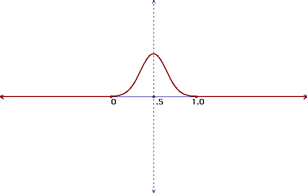
Related to the idea of proportions in a population is the symmetry of the normal distribution. The proportion of values that fall to the left of a certain point within the distribution, which represents the area under the curve from that particular value to the left, can be represented by labeling the normal distribution from 0 to 1 with the mean of the distribution at .5 as shown below:

Z-statistic
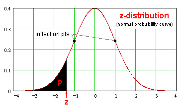
We have learned that certain proportions of the data set fall within certain areas of the normal distribution. The z-statistic, similar to the proportion distribution, relates certain values to their distance from the mean in a given data set. The z-statistic is directed, with values to the left of the mean being negative and values to the right of the mean being positive. The mean has a z-statistic of zero. The value in the data set that is one standard deviation higher than the mean has a z-statistic of 1, and the value one standard deviation below the mean has a z-statistic of -1. Similarly, a value two standard deviations higher than the mean has a z-statistic of 2 and a value two standard deviations lower than the mean has a z-statistic of -2. The distribution of the z-statistics for a normal distribution is shown below:

There is a table of values that relates the z-statistic with the corresponding probability that a value lies to the left of the value that correlates to that z-statistic. This table is known as the z-table. Values having a z-statistic of 0 are equal to the mean and therefore the z-table value is .5, indicating that there is a .5 probability that other values from the data set will lie to the left of that value. A value having a z-statistic of 1 has a z-table value of .8413, indicating that there is a .8413 probability that other values from the data set will lie to the left of that value. This represents the half of the distribution that lies to the left of the mean as well as the 34% (half of 68%) of the data that lies between the mean and one standard deviation above the mean.
When a sample of data approaches a normal distribution, a z-score
for a particular value can be calculated and used to approximate
the probability of an event occuring based on the z-statistics.
If x is an observation from a distribution that has a mean ![]() and a standard deviation s, then the
z-score for that value is:
and a standard deviation s, then the
z-score for that value is:

Probability and the Z-statistic
The z-statistic for a value in a data set can be used to predict the probability that other values in the data set will be above or below that value. For data distributions approaching the normal distribution, a value in the data set, the mean of the data set and the standard deviation of the data set can be used to calculate the z-score for that value. The z-score is an estimate of the z-statistic, which will indicate the probability that other values in the data set are lower than the value with the given z-score.
For example, if the mean of a data set was 10 and the standard deviation was 2, then the z-score for a value of 13 would be 1.5. Using the z-table, we find that this z-score correlates to a probability of .9332. This means that there is a 93.32% chance that a value from this data set will be less than or equal to 13.
The teacher should have the students work with different data sets to determine sample proportions and/or z-scores for certain values in those data sets.
Now that you have an understanding of proportion and the z-statistic for the normal distribution, go back and look at Carl's height data for his other two pitchers (from Lesson 2). If he doesn't mark those pitchers to ensure appropriate drink strength, what will be the probability that a mixture from each of the other pitchers is sufficiently strong?
Edith from Lesson 3 has decided on the weekly quantity of blueberries she will order to make the blueberry pies for Patrick's Pie Patch. Click here to see her data from filling the pie plates with blueberries. She will purchase 2.08 tons of blueberries weekly. If there are 500,000 blueberries in each ton and Patrick has a demand for 2,500 blueberry pies each week, will Edith have ordered enough blueberries? How sure are you?
The class should perform some calculations and discuss their answers.
The z-statistic correlates to a certain area under the curve
to the left of the value with that particular z-statistic. This
area under the curve represents the probability that other values
in the distribution will be lower than the value with a given
z-statistic. Related to the z-statistic is the critical value
z*, which represents the z-statistic associated with a given area
under the upper tail of the normal distribution, or the probability
that a value is higher than the value with the given z-statistic.
When the standard deviation of a population is known but the mean
is not, then a sample mean can be used to estimate the population
mean to a desired confidence interval. Using a table that correlates
desired confidence level (or probability) to a z* value,
the sample mean ![]() can be used to
estimate the population mean m using
the following formula:
can be used to
estimate the population mean m using
the following formula:

where s is the population standard deviation and n is the number of values in the sample.
Cofidence Intervals - sample proportions
When information about the entire population isn't known, then
the probability of a given occurrence or value must be determined
using proportions. Using the z* value mentioned before,
the proportion of the population (p) can be found to a certain
confidence interval by using the sample proportion ![]() and the following formula:
and the following formula:

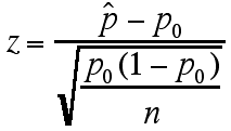
Similary, to use a sample proportion to test the relationship between the population proportion (p) and some hypothetical proportion p0, the hypothetical proportion is used to calculate a z-statistic and then use this to determine a P value (probability relating the hypothetical proportion to the population proportion) using the following formulas:

Probability that p0> p is  ,
where p(z) is the probability associated with that z-statistic
Probability that p0 < p is  ,
with p(z) same as above
Probability that p = p0 is  , with p(z) same as above
The teacher should provide an example with a known population standard deviation and a sample mean to determine a confidence interval for the population mean. Several examples of data samples should be examined against some hypothesized proportion to determine the probability that the population proportion is greater than, less than, or statistically unequivalent to the hypothetical proportion. They also should determine some proportion confidence intervals for poplulation proportions based on sample proportions.
Click here for table of positive z values
Click here for table of negative z values
Click here for table of z* values
Charlie has decided to use Lucy's data to determine the packaging weight for the Nutty Swirl bar from Lesson 1. He is planning to put a value of 2.05 grams on the label for every bar. Charlie doesn't realize that Federal regulations require that his product meet or exceed the label value for weight 95% of the time. Is Charlie breaking the law?
Now you have all the tools necessary to function as the quality control engineer for Sunshine Sugar Factory. Determine how best to allocate the production lines for Sunshine's major customers and justify your decisions in terms of statistics.
Click here to see some discussion of the solutions for the lesson problems and the unit problem.