Methods for Finding Roots of Functions

by Mark Freitag

Functions are one of the fundamental concepts in mathematics. So many situations and applications can be modeled or represented by them that a large portion of mathematics taught in high school and college are topics that deal with fucntions. One very nice thing about functions, is that once we have a situation represented by a function, we can use the rule to predict or evaluate other values. Let me clarify this using a concrete example. Suppose I have a situation that can be represented by the rule f(x) = x^2 + 5x, and I want to know when this function will equal -6. (i.e. -6 = x^2 + 5x) In this case all I need to do is move all terms to one side of the equation and have 0 on the other side. From here it is a simple matter to solve the equation by factoring.

-6 = x^2 + 5x
0 = x^2 + 5x + 6
0 = (x+2)(x+3)
x = 2 or x = 3

So this rule will equal -6 when x is either 2 or 3. This particular situation has many applications, but to list these applications is not the purpose of this essay.

High school students spend much of their time learning to manipulate variables and expressions in order to find the roots of the function. But unfortunately, the functions that they will encounter in their occupations are very rarely nice. In fact, it may be the case that most of the functions they deal with will not be factorable or easily manipulated. Take for example the function f(x) = .5e^x - 5x + 2. How can a highschool student go about finding the roots of this equation. Most likely, in these cases an estimate of the root with accuracy to a certain number of decimal places will be sufficient. This esitmation could be very difficult if not impossible to do by hand, depending on how the student is at calculus and calculating numbers. A mcuh better way to handle these situations is to use technology. This essay will demonstrate four different ways to find the roots of equations. Only one will not be applicable to high schools students who ave not had calculus. Throughout this demonstration I will be finding the roots of

f(x) = .5e^x - 5x + 2.

Using Graphs

One of the easiest ways to estimate roots of a function is to graph the function using technology and then "zoom" in on the root. There are many different graphing programs that will do this, and even graphing calculators (TI-82), which might be the most available technology, can so this. In this essay I will use the program Algebra Xpressor.

To begin simply graph the equation y = .5e^x - 5x + 2.

Hence from this graph we can see that this is indeed a function, and that it has two roots in [0, 5]. We can estimate the roots to be about 1 and 3, but this is not very precise. To improve the precision, we can use the technology to zoom in on one root at a time by changing the axes. If I consider the larger root first, I can "zoom in" and obtain the following graph.

From this picture we can see that the root is just larger than 3.4. To obtain more precision, I can zoom in again, and I can continue this process until I reach my desired precision or the precision on my machine becomes inadequate. The next several graphs show estimates of the larger root up to the precision of the machine.

So, by this last graph, we see that the larger roots is approximately 3.401795803857806749. This gives us accuracy to 17decimal places. Again most students should be able to do this with no problem. The same thing can be done to approximate the smaller root.

Bisection Method

The second method that I will demonstrate is the Bisection Method. This method can be used with either a spreadsheet or a graphing calculator with spreadsheet capabilities. Basically, the bisection method squeezes in on the root from both sides by making use of the Intermediate Value Theorem. In essence, this theorem says that if f is a continous function on [a, b] and the sign of f(a) is different from the sign of f(b), then there must be some point, c, in the interval such that f(c) = 0, and is thus a root of the function. The Bisection method uses this to squeeze in on the root in the following way. First, we can select an interval that contains the root we are looking for by looking at the graph. Second, we find the midpoint of the given interval, in this case (b - a)/2 = m, and then look at the function f evaluated at a, b, and m. Third we compare the signs of f(a), f(m) and f(b). f(m) will be one of three things. It will either have the sign of f(a), the sign of f(b), or it will be 0. If it is 0 (it usually isn't), then we stop because we have found the root we are looking for. Now, suppose that the sign of f(m) is equal to the sign of f(a). This implies that the root will be between m and b, and so we choose [m, b] as our new interval and repeat the process. Similarly, we replace b with m if the sign of f(m) equals the sign of f(b). Which ever the case we know that the root is in our new interval, and the endpoints of that interval have different signs. To "squeeze" in on the root we continue the process, until the desired accuracy is achieved.

I used the progarm Excel to find the roots of the equation f(x) = .5e^x - 5x + 2. I obtained the following results.

So, after 24 iterations we see that the smaller root can be found in the [.578300476, .578300595]. So we can estimate one root to be about .5783005. One of the first things to be noticed about this process is that it takes a lot of iterations to get a high degree of precision. It might be asked, is there a way to get the roots in fewer iterations. Well, as a matter of fact there is.

Newton's Method

There are in fact two ways of getting the similar results in a shorter number of iterations, Newton's Method and the Secant Method. Unfortunately, you need to know some calculus for Newton's method, and so it may not be appropriate for some high school students. Anyhow let me give you a brief description of how Newton's method works. First, we must make the assumption that the function, f, is differentiable on [a, b]. If it is, then f will have a definite slope at every point in [a, b]. Let (c, f(c)) be a point on the curve where c is in [a, b], so there is a tangent line at this point which is an approximation to the curve at that point. We can describe this line by

l(x) = f'(c)(x - c) + f(c)

Now we can take the zero of this line as an approximation to the zero of f. This zero can be represented by (c' represents the zero)

c' = c - f(c)/f'(c)

We can now take the point c' as our starting point and repaeat the process. In this way we get a sequence of values that come closer and closer to the root of f. Maybe the following picture will help.

Since this process can be done with iterations, we can attempt this process using a spreadsheet. I have found approaximations of the two roots of f(x) = .5e^x - 5x + 2 using several different starting values. In the first data set, I started with x = 0 and then x = 1. It can be seen that in both trials I found the root to be approximately x = .578300577, which agrees with our earlier approximations.

In the second data set, I started with x = 3, x = 3.5 and x = 4. In all three trials, I found that the root is at approximately x = 3.4017958.

To set up the spreadsheet to do this algorithm, let x be the starting value and let the spreadsheet compute f(x) and f'(x). Then simply let your next x-value be x - f(x)/f'(x). Simply drag down in all three columns and let the computer do the work.

Unfortunately, there are some problems with Newton's method aside from the fact that the student must know what he derivative is. First, the x-values may run away in a sense (a). This might occur when the x-axis is an asymptote. Hopefully, the picture below will clarify this. Second, we might choose an x-value that when evaluated in the derivative give us 0 (b). The problem here is that we want the tangent line to intersect the x-axis so that we can approximate the root. If x has a horizontal tangent line, then we can't do this. Third, we might choose an x, that is the beginning of a cycle(c). Again it is hoped that the picture will clarify this.

Now, if your students don't know calculus there is a method similar to Newton's method, only it does not use the derivative of a function.

Secant Method

The method here relies on the same idea, only instead of using tangent lines, we use secant lines. (See the picture).

So, for this method we will need two intial guesses and our iteration revolves around the use of two numbers. The nice thing about this, is that we do not need to know the derivative of the function, since we can set up our iteration in the following manner.

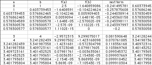
Again, using a spreadsheet makes our computations easier and quicker.

Again, it can be seen that we achieved "good" approximations of the two roots. (Look in the last entry in the b column for the approximation), and it took considerably fewer entries than the bisection method.

I have found the roots to only one funtion, but these methods should be of use with almost any continous function. Since functions play a large role in the high school and college curriculum, it is hoped that these four methods of finding roots can be of use to teachers.

Pictures for Newton's Method and the Secant method were obtained from Cheney and Kincaid (1994).

References

Cheney, W. & Kincaid, D. (1994). Numerical Mathematics and Computing. Brooks/Cole: Pacific Grove, CA.

Return to Mark Freitag's Homepage