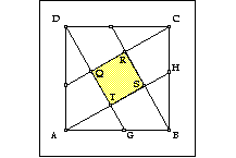
Figure 1

Our first reaction was to analytically determine the area by using what
we knew about similarity and, naturally, we focused on the following algebraic/geometric
method.
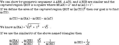

So, we have an answer and what may be considered a complete solution. Clearly,
this is a paper trail leading to a numeric answer where organization and
logic are important but this single case leaves many questions unanswered.
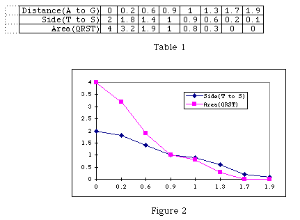
As G moves along segment AB, side TS and the captured area decreases.
We tried to predict the nature of these decreases. This notion emerged from
our discussion regarding the selection of points where data was collected.
We made no attempt to collect data at uniform distances nor were we particularly
concerned about precision at this point. The data poorly illustrated rate
of change so our next move was toward a graphical illustration (Figure 2).
It was clear, at least under the level of precision we used and from Figure
2 neither the side nor area of the captured region changed at a constant
rate.
Recall, we had not yet looked at the algebraic model for this phenomenon.
We assumed the irregularity of side measures was attributable to the level
of precision set within the software. With this in mind, we assumed a constant
rate of change for the side measure but our intuition left us with a suspicion
further investigation was required.
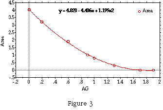
Likewise, we assumed quadratic definition for the rate of change of area
for two reasons. First, the plot in Figure 2 approximated a segment of a
parabola and second, area is considered the product of two linear conditions.
Our graphical model in Figure 2 left us with a decision about whether our
representations were precise enough and whether our assumptions were justifiable.
We had two choices to help determine whether our assumptions were on line.
One choice was the creation of a curve of best fit for each set of data
and compare the results found from their algebraic definitions. The second
choice was a more efficient choice, it called for the development of defining
functions for side measure and area from the our original numerical solution.
We knew which choice was most efficient but we wanted to authenticate our
assumptions, so we chose to find curves of best fit (Statview) and their
corresponding functional definitions.
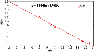
Statview software regressed to a linear function representing the measure
of side and a quadratic function for area. In both cases, the algebraic
models were rather precise (mean error 0.0005). Under normal circumstances
this solution may have been accepted as complete but as we said earlier
our intuition about fairness of representation and precision led us to ask
a follow-up question. How fair are algebraic and geometric models if we
choose to extend AG beyond B in a positive direction and beyond A in a negative
direction? There were some clear problems. The geometric model indicated
as AG grew beyond B to the right there was a point where area and side increased
in size but tended to a limit. This was the first inconsistency since our
models (linear, quadratic) indicated unbounded side and area measures as
AG increased. Similarly, as G moved beyond A to the left there was also
an upper limit for both side and area measures. In addition, the rate of
change of side and area measures appeared different if one were to compare
the activity of the geometric model when G was moved left or right. Clearly,
our curves of best fit were useful but limited.
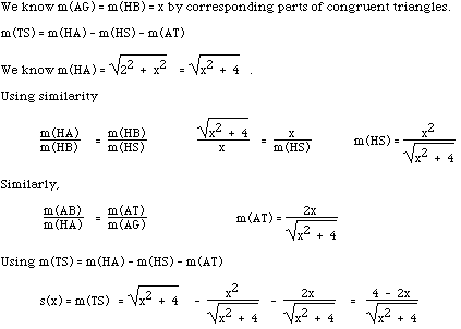
So the concern for a higher degree of precision and fairness led us back
to the derivation we developed in answering the original question. We assigned
x to represent the value of m(AG), s(x) to represent the side measure, and
f(x) the area of the captured region QRST. The following s(x) and f(x) resulted.
![]()
It is immediately clear these functions are not of linear or quadratic form
so we decided to correlate our collected data to values generated from s(x)
and f(x) and found r = 0.9995. Again, we were satisfied with the precision
and now more confident about the fairness of our model. The basis of our
confidence was rooted in the logic of our symbolic derivation and the improved
correlation. We felt our confidence would greatly increase if we could make
predictions beyond the interval ![]() . This led to a next phase of our
solution by releasing the restriction of G to the side of a square. Why
not let G ride along a line AB? The first test was to use our improved s(x)
and f(x) and plot them over a domain
. This led to a next phase of our
solution by releasing the restriction of G to the side of a square. Why
not let G ride along a line AB? The first test was to use our improved s(x)
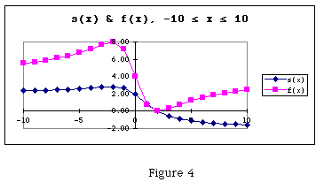
and f(x) and plot them over a domain ![]() which resulted in Figure
4.
which resulted in Figure
4.
The plot of s(x) indicates an increase in s(x) from x = -10 to x = -2 and
then there is a relatively sharp drop to where s(x) = 0 then it somehow
becomes negative. Once s(x) becomes negative it appears the rate of change
in s(x) decreases and possibly approaches a limit. Figure 4 promotes many
questions. What does a negative s(x) (side measure of the captured region)
mean? Is there a limiting value for s(x) and if so what is the value? In
a likewise fashion, f(x) increases from x = -10 to x = -2 where a maximum
occurs and then decreases at a quicker rate to a minimum of f(x) = 0 when
x = 2. Once past x = 2, f(x) increases and also tends to a limit. This is
consistent with what happened to s(x) and if the side of the captured region
tends to a limit it is reasonable for the area captured to have the same
characteristic. As with s(x), the graph of f(x) suggests questions such
as:
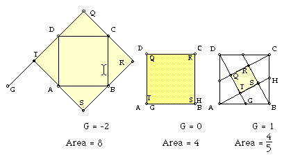
The algebraic and graphical representations told a story but the newly generated questions certainly had merit and we felt deserved pursuing. We felt there was a compelling reason to push one step further. If software permits a pictorial model then why not build more confidence into our algebraic and graphical models with a geometrical model. The original Geometer's Sketchpad model was altered to accommodate the movement of G and the sequence of pictures in Figure 5 resulted. The questions addressed through the extended Geometer's Sketchpad model aimed at addressing the questions:
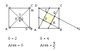
The second question, Is there a limiting value for s(x) and if so what
is the value?, can also be addressed and with varying degrees of sophistication.
A less sophisticated discussion may only include a comparison of pictures
representing areas of 4/5. In one case (G = 1), G is only one unit from
where area = 0 and in the second case (G = 4), G is 2 units from area =
0. This suggests that it has taken s(x) a longer time to grow back to its
previous size. In addition, when the model was extended such that G moved
a great distance from A the data in Table 2 resulted.
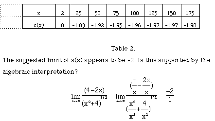
What about the question relating to area (f(x))? Can a maximum area of
8 be justified? Justification of a maximum area can be a calculus or geometrically
supported case. From calculus, recall the notion of using a first derivative
set to zero (the regions on a curve with zero slope).
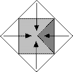
This is normally the practice when such a question is asked but in our
case the geometric model illustrated just one case when the captured area
had an area at 8. To reaffirm the area was 8, we flipped in the flaps indicated
in Figure 6. This provides sufficient evidence for current purposes.
If there is a story to be told then it seems the focus here was based on
the construction of a net of observable and justifiable connections. There
are many more questions, answers, and justifications to be found in such
a problem but the important factors are the generation of ideas promoted
by collaborative efforts and the understanding needed to connect models
used to communicate mathematics. Some models seem fair but limited. It is
important to recognize limits and extensions when necessary and there must
be a willingness to deviate traditional solutions. Maybe, technological
tools need to be used as vehicles for illustration and provocation that
enrich mathematical solutions. State and national Standards recommend richness
of solution for future school mathematics so it seems appropriate to use
what we know and question where it fits in coming to better understand what
is learned. This suggests understanding mathematics based on at least two
levels. One level recognizes detail and logic holding a solution together
and the second level, suggests a more holistic view. A view that locates
a problem solution in a context and illustrates inter and intra relationships
between elements of the solution and that context.