Chapter 5: Probability Theory

Section 5.2: The Binomial Distributions

The binomial setting

1. There are fixed number of observations (n).
2. The n observations are all independent.
3. There are only two possible outcomes for each event: success and failure.
4. Probability of success, p, is the same for each trial.

The distribution of the number of successes, X in a binomial setting is called a binomial distribution with parameters n and p. The possible values of X are whole numbers from 0 to n.

Binomial probabilities

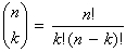
Binomial coefficient: the number of ways to select k objects from n total objects. This is represented by . This is calculated by: , where n! = n·(n–1)·(n–2)····2·1 and 0! = 1.

Luckily, we can perform this calculation on the TI-83 calculator!

Binomial coefficient: If X has the binomial distribution with n observations each with probability, p, of success, then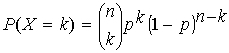

Again, we can perform this calculation on the TI-83 calculator!

Binomial mean and standard deviation

If X has the binomial distribution with n observations each with probability, p, of success, then
μ = np

The normal approximation to binomial distributions

For large n and for p near 0.5, the binomial distribution can be approximated by a normal distribution. More specifically, we can use the normal approximation the the binomial distribution if the following conditions are met:

1. np ≥ 10
2. n(1 – p) ≥ 10