Graphic Solution

Ken Montgomery

EMAT 6690

MATHEMATICS APPLIED IN INDUSTRY

Linear Programming: Graphical Solution

A company produces two types of product (Gadgets and Gizmos). The manufacturing process consists of assembly, polishing and packaging. The time required for each stage of manufacturing, for each product is given in Table 1.

Process	Gadgets	Gizmos	Total Time Required
Assembly	2	4	36
Polishing	3	1	36
Packaging	5	2	30

Profit	$30	$20	-

Table 1: Production Time Requirements

We let andrepresent the numbers of dozen Gadgets and Gizmos, respectively and thus obtain the objective function (Equation 1) for profit, which we desire to maximize.

Equation 1:

From table 1 we obtain the following production constraints.

We also assume that production capability (parts, labor, etc.) will never be negative, so we satisfy the following necessary inequalities.

To solve this problem using the graphical method, we begin by first graphing the system of inequalities. We plot these inequalities one at a time, to better understand how the constraint space is developed. Figure 1 shows a graph of the first inequality.

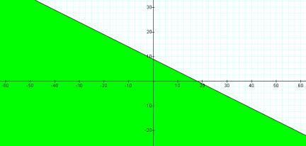
Figure 1: Graph of

Graphing the second inequality on top of the first yields the composite graph in Figure 2.

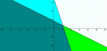
Figure 2: Graph of and

Our constraint space begins to take space as the darker, bounded intersection of these two inequalities. Graphing the third inequality on top of the first two yields the composite graph in Figure 3.

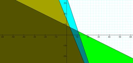
Figure 3: Graph of ,and

In Figure 3, we have the final composite graph of the three However since we also have the inequalities and, our constraint space is further confined to only the positive region of the bounded region above. This final constraint space is given in Figure 4, with andplotted in yellow, on top of the previous three inequalities.

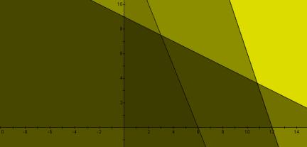
Figure 4: Composite graph of ,,,and

Notice the darkest region of the graph, a quadrilateral with vertices (0,0), (0,9), (6,0) and (3,7.5), which is the bounded constraint space. Testing each of these vertices in turn we obtain four possible values of z, given by the following four equations.

Testing values inside the constraint space will demonstrate that 240 is the highest z-value. To understand why the maximum z-value must correspond to a vertex we plot the objective function over our constraint space.

We next plot the objective function for profit. However, this equation is in three variables, representing a plane and requiring a three-dimensional plot. Nevertheless, the above graphs each represent the x-y plane, and the intersection of the objective profit plane with the x-y plane should be a line, which we can then plot in our present perspective.

Solving the objective profit equation for y, in terms of z provides an entire family of lines with the same slope and with y-intercepts that are related to the value of z (Equation 1).

Equation 1:

You may download the Graphing Calculator file Gadgets&Gizmos.gcf to explore this parameterization in z or view the Quicktime movie Gadgets&Gizmos to see the dynamic representation of this family of lines.

The only corner or vertex of the constraint space below that the line touches is given by the values x = 3, y = 7.5 and which correspond to the z-value of 240. Notice that the line passes through the point at this corner of the constraint space illustrating this optimal value of z for the parameterized line equation and thus for the plane equation (Figure 5).

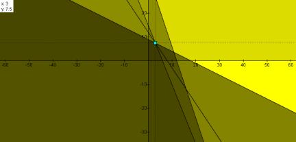
Figure 5: Objective function plotted with optimum z-value

Notice that if the objective function (Equation 1) were plotted so that it passed through another vertex or points inside of the constraint space, these lines would have lower y-intercepts and since there is a direct, linear correlation between the y-intercept and z (i.e. ), a lower y-intercept corresponds to a lower z-value or profit. Figure 6 provides a plot of the objective function minus the yellow, overlaying constraints of positive x and y values for contrast.

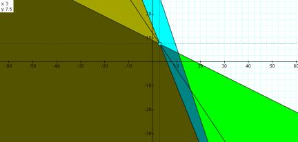
Figure 6: Plot of objective function over constraint space without andconstraints

Return to EMAT 6690