
The following problem was given to explore and write up. Given a rectangular sheet of cardboard 15" by 25 " if a small square of the same size is cut from each corner and each side is folded to form a lidless box find the following:
A. What is the maximum volume?
B. Whate size(s) of the square would produce a box of volume 400 cubic inches?
C. Prepare a demonstration or solution using GSP, Algebra Expressor, etc.
A. To determine the maximum volume we first need to determine the dimensions of the box then simply find the polynomial which represents this volume and find its maximum. I began by making a GSP model of the lidless box to determine the diminsions. See the box below.
From the diagram one could estimate appropriate values of x. For instance we know that x cannot be 10 because this would give a negative width. In fact it seems the maximum x would at least have to be less than 7.5 as this would give the degenerative case in which the width would be zero. Upon further investigation if we look at the curve that is generated by this volume ie.
![]() we see the maximum value of x is
somewhat smaller than our estimate of 7.5. Below using MacNumerics I will
show the curve. Note the maximum occurs at approximately513.0513 cubic inches.
This maximum will occur when the x value is approximately 3.034. The graph
will show an estimate if we trace the curve to its highest point. Another
way to solve this in class would be to use the graphing calculator. I would
suggest students trace the maximum so that they conceptually understand
what a maximum looks like graphically. The graphing calculator will actually
calculate the maximum for them, but I find that often this is simply button
pushing and a black box effect until they have actually traced the highest
point for themselves. Then the calculator can be used to aid them in accuracy.
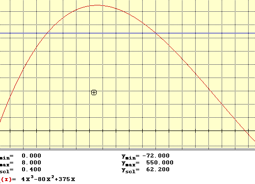
On the MacNumerics program I have used General Functions and Polynomials
to graph this polynomial. Both programs allow for exploration and tracing.
See below.
we see the maximum value of x is
somewhat smaller than our estimate of 7.5. Below using MacNumerics I will
show the curve. Note the maximum occurs at approximately513.0513 cubic inches.
This maximum will occur when the x value is approximately 3.034. The graph
will show an estimate if we trace the curve to its highest point. Another
way to solve this in class would be to use the graphing calculator. I would
suggest students trace the maximum so that they conceptually understand
what a maximum looks like graphically. The graphing calculator will actually
calculate the maximum for them, but I find that often this is simply button
pushing and a black box effect until they have actually traced the highest
point for themselves. Then the calculator can be used to aid them in accuracy.
On the MacNumerics program I have used General Functions and Polynomials
to graph this polynomial. Both programs allow for exploration and tracing.
See below.
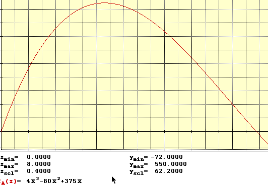
Note the scale for the x values is .4 and the y scale is 62.2. While the student can trace on this program the picture feature does not capture the trace bar. When tracing we find that the maximum occurs when x is approximately 3.034. Of course a complete graph of this curve could be useful in discussing how x could not be particular values because the y values become negative and since the y represents a volume here the student could see a nice graphical depiction of why x cannot be certain values.
B. In exploring question B to find the size of the square that would produce 400 cubic inches we find that there is more than one solution to this problem. One technique that can be used is to graph the polynomial representing the volume and then graph the line y = 400 and find the intersection points. This is a particularly effective method on a graphing calculator. It also works on MacNumerics. See below.
Of course a rough estimate could be made for the intersections. Remember the scales for the graph when making estimates. One can see that there are two intersections and therefore two values of x which will work since both x values fall in a small enough range to fit the constraints of the problem. Approximate values for x are 4.7928 and 1.5249. When these values of x a put into the expressions which represent the sides of the rectangular box we will find the dimensions. An estimate of the dimensions are 5.4144 by 15.4144 by 4.7928 and the second case in which we find 11.9502 by 21.9502 by 1.5249. Each of these cases when multiplied yield an approximate volume of 400 cubic inches.
Additional questions that one might ask could include what do the roots to this polynomial represent? What is the maximum area that this rectangular box might have? Model the area as the graph of a curve. etc.
A second question to consider was given as follows: Consider triangle ABC. Select a point P inside the triangle and draw AP, BP, and CP extended to their intersections with the opposite sides at points D, E and F respectively. Explore (AF)(BD)(EC) and (FB)(DC)(EA) for various triangles and various locations of P. Make conjectures. Prove? Can the results be generalized?
First we will look at a GSP drawing to determine any relationships that can be measured.

I will show several locations for P. Note each time the products remains equal and the ratio of course remains constant.


It was interesting to note that if P is on one of the vertices the products resulting is zero. To further explore this click here for a GSP drawing.
I have selected for my exploration not written up previously an extension of my Write Up Eleven.
Click here for Elevenextension.
I would like to use my discussion on Assignment 11 as the assignment in which I learned the most mathematics. I have had limited study and/or exposure to the concepts in the polar equation format and I found it intriging. It seems the high school curriculum circumvents this type of discussion, and therefore I have had no opportunity to teach or study these curves in a number of years. I am most satisfied with my presentation on this assignment because I think I was more thorough in my investigation, and because I think there was definitely a steep learning curve regarding how a write up should be presented. I think my earlier efforts were lacking in thoroughness and in inspiration. It takes free time unfettered from other demanding situations to feel the freedom to simply explore and enjoy the exploration. I found this time only after my obligations as school were satisfied, and I could concentrate over the holiday break period. I think this write up was presented logically and flowed naturally as my own investigation did. I found myself engaged and curious about how the changes in the equations might be predicted. Sometimes I could predict the outcome, but often I could not. I am pleased with the overall outcome of this project. Click here for Assignment 11.
I also feel that my one of my most creative works during the quarter was in Assignment 10. (Click here for Assignment 10.) I was able to explore different elements of parametric curves than I use in a high school setting. We seldom graph parametrics at least to this extent. Typically in the curriculum one teaches students how to eliminate the parameters and possibly introduces a few simple graphs done by hand. Now with a computer environment which would allow the student to explore many graphs in a single class period I would hope these curves could be discussed in greater depth. Students are rarely given a chance to simply go to the computer lab and explore. There is usually an agenda of finding a particular theorem or conjecture for the day. There is little time, if ever, that they are simply asked to make as many conjectures as they might find. I must admit that unknowingly I have typically used the objectives as a restraint to open exploration, but there is no reason why I cannot change this aspect of my teaching. Of course there is a time constraint and the limited use of a computer for some students will inhibit their freedom and creative explorations.
There is not just one assignment in which I felt that I learned the most mathematics. However, one assignment that caught me off guard was Assignment 7 ( Click here.) At first I did not recognize that I was constructing an ellipse. After making the construction, however, I explored how changing the center of the smaller circle internal to the larger one would satisfy the definition of an ellipse. Further I found that once the center of the smaller circlewas moved exterior to the larger circle the fixed differences between the centers satisfied the definition of an hyperbola. This assignment was a very interesting one.
The exercise that opened new elements of mathematics to me was one which upon first reading I thought I already have a great deal of experience with this topic. As often as I have worked with quadratics I have never seen the approach of this particular lesson in Assignment 3. (Click here.) It has not occurred to me to have students look at the xb plane or the xc plane. I think this would be very helpful to students algebraically, and I also think it might help their understanding of the notation f(x). They usually memorize that the vertex can be found by finding -b/2a for the x coordinate and replacing that value for x in the expression yields the y coordinate of the vertex. But having them look at patterns and realize the vertex is at ( -b/2a , f ( -b/2a) ) is a worthwhile exercise. Also simply obtaining values in the xb plane will enhance their viewpoint of the graph and demonstrate more algebraic skills as well as geometric understanding. One concern I have in the new curriculum is the lack of rigor in their algebraic manipulations. Many students now can discuss, explain and conjecture, but algebraic manipulation that we took for granted 5 years ago in no longer there. (I wonder if you will find this to be a problem in your undergraduate students in the next few years.)
Overall this semester I have learned a great deal of new ways to approach the mathematics that I teach. I used the spreadsheet and geometric sequences in musical instrument in my class. In fact the students jumped at a chance to bring in their instruments and I enjoyed their jam session at the end. Unfortunately we did not have a mandelin player amoung the group. I appreciate the alternate ways to present concepts to students and the opportunity to explore some on my own. My own personal circumstances prevented me from having the time that I would have liked to contribute, however I know I will use many of these ideas in the future to explore my own learning and to enhance my teaching. Thank you for an interesting quarter.
Click here to return to Sandy's Home Page.