Spring problem
November 15, 2010
This investigation looks at how to create a model that fits the movement from a spring.
Please note: you might need a plugin to play the animations in this page.
1. The Problem
2. The Data
4. The Result
1. The Problem
Here's an animation of the problem we're dealing with:
A spring is attached to some object and pulled downwards, the spring in our problem is a bit simpler because it doesn't a have a weight attached to it. A very sensitive sensor was used to record the height of the spring as it moved up and down. This data was recorded and captured in this excel spreadsheet.
2. The Data
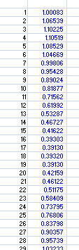
The data looks as follows: 296 sets of (x,y) where x is the moment in time and y is the height of the bottom of the spring e.g.
(1,1.003)
(2,1.06)
(3,1.12)
(4,1.06)
...
...
(296,0.77)
Here's a screenshot:
By selecting both columns and selecting insert chart, we get the following:
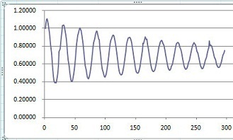
This ability to graph the data is very useful in attempting to model it because we can see what it looks like. Remember that the data is not continuous, it's actually just several dots that overlap.
3. The Modeling Process
Here are some important things to notice when creating our model:
- The data is periodic, so we'll probably need some trigonometric function.
- The amplitude decreases over time, which is something that a trigonometric function can do on it's own.
- The decrease in amplitude doesn't seem to be linear, so we'll go with an exponential function.
- The data is not centered around 0, it's moved up a bit.
So let's get to it:
Here is a look at the sine and cosine graphs:
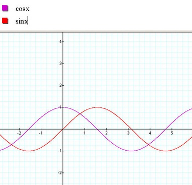
Cosine is a better fit because our data also starts high and then lowers as opposed to sine that starts at zero and moves upwards.
The next problem is that the data doesn't centere around zero like cosine so we need to move it up a bit.
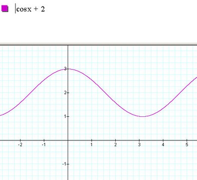
Now let's look at the exponential function:
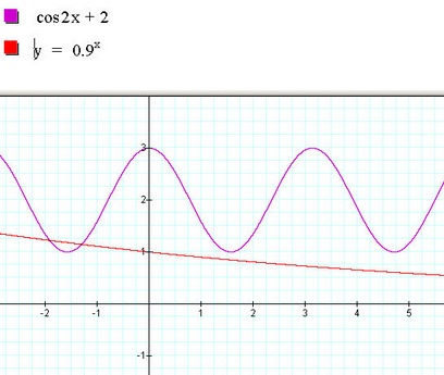
The exponential function decreases nice and gradually so let's put these two together and see what happens:
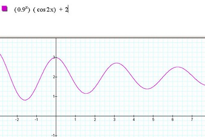
By simply multiplying the two functions together we get a cosine with a decreasing amplitude.
If we look at the top function, we get an idea of what needs to be done, consider the following:
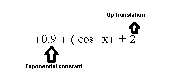
We need:
- a constant for the exponential function (which proved to be the trickiest!),
- a translation upwards, and
- someway of getting the domain of the x-values (1 up to 296) into something that is more compatible with the consine function.
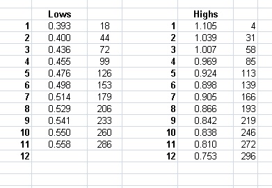
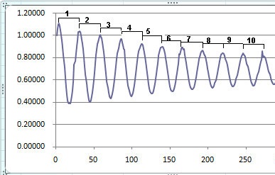
The points we need to consider for the exponential fit are illustrated here:
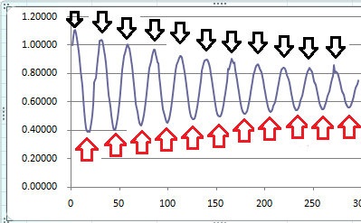
The black arrows indicate the high points (relative maxima) and the red arrows indicate the lows, or relative minima. If we can seperate this from our list of data, then we can simply use an excel function to tell us what the constant should be.
Take, for instance the data {1,2,3,4,3,2,1,0,1,2}, it has 10 elements and we want a function that isolates the 4 (high) and the 0 (low).
Consider the following:
(1-2) times (2-3) is negative times negative which equals positive,
(2-3) times (3-4) is the same, but
(3-4) times (4-3) is negative times positive which equals negative,
in the same way
(1-0) times (0-1) is also negative
This property (the product's sign being negative) is unique to the high and low points. So in excel we can achieve this with:
=IF((C32-C33)*(C33-C34)<0,C33,0)
This basically means that if the product is negative, display the value where it occured:
Now we can take all the high points and low pionts and put them in two tables with their x-values:
Using the LOGEST function in excel, we get the constant we needed , like the 0.9 used in the example in section on finding the right functions.
It's really too easy to get this one using excel:
We just need take the average of the one and the inverse of the other (1 - LOGEXP). Now that we have the exponential constant, let's look at the cosine function. Let's first look at the period:
The x-value at the start of the first period is 4 and at the end of the last period is 272. So we simply take the difference and divide by the 10 periods:
(272-4)/10 = 26.8
Now that we have this, it's easy to convert to what the cosine needs: it's period is about 6.28 or 2 pi, so we take whatever the x-value is, divide it by 26.8 and multiply by 2 pi.
Lastly, we need the translation upwards. The most straightforward approach is to take the average of all the y-values over one or several complete periods. This value is 0.7210.
In this video, the exponential constant is a bit off so we simply adjust it gently using 100 000th's of a unit and picking the best fit by inspection:
4. The Result
So our model looks like this:
f(x) =
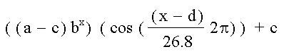
- x : values in the left column of the data
- a : exponential function coefficient
- b : exponential function base
- c : horizontal shift
- d : vertical shift
Substituting the values from excel we get:
f(x) =
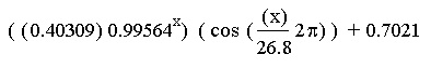 This
model can now be used in stead of the data table to estimate the
position or amplitude of the spring at any given time.
This
model can now be used in stead of the data table to estimate the
position or amplitude of the spring at any given time.